Figure 3.

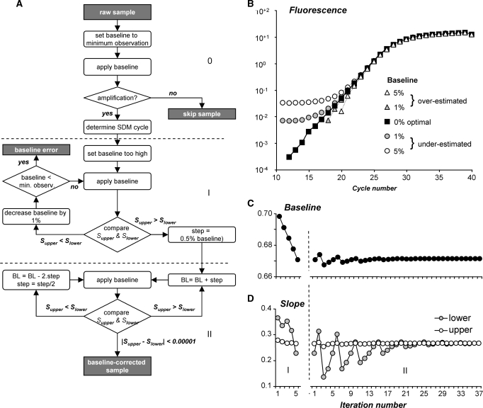
Fluorescence baseline estimation. (A) Flowchart of the baseline estimation algorithm. For each sample, an initial baseline is set to the minimum observed fluorescence. Samples are skipped when less than seven times increase in fluorescence values is observed. For each sample that shows amplification, an iterative algorithm than repeatedly adjusts the baseline value until the slope of the regression line through the data points in the upper half of the exponential phase differs less than 0.0001 from the slope of the line through the data points in the lower half. At a PCR efficiency of 1.8, this criterion translates into an efficiency difference of 0.0004. The algorithm results in a set of data points on a straight line and effectively reconstructs the exponential phase. (B) Comparison of amplification curves resulting from an optimal baseline (filled squares) with the curves resulting from 1% to 5% over-estimated (gray and open triangles) and 1% to 5% under-estimated baselines (gray and open circles) showing that the shape of the curves is dependent on the baseline estimate (21). This change in shape of the curve is used to estimate the optimal baseline (A). (C) The graph shows the baseline values in both phases of the baseline estimation. (D) The graph shows the slopes of the regression lines through the upper (S_upper) and lower (S_lower) halves of the continuous set of data points in the exponential phase when the baselines in (C) are applied.