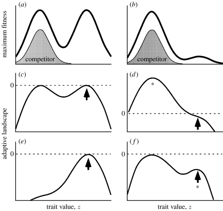
Figure 1.

(a,b) Maximum individual fitness plotted as a function of the trait value z, reflecting the resource distribution in the environment. Resources associated with the right peak are (a) abundant at the range centre and (b) very low at the range edge. Fitness is calculated as w(z)=exp{r^max(z)}. The shaded area shows the phenotypic distribution of the competing species at its evolutionary equilibrium. (c–f) Adaptive landscapes for the focal species (i.e. the one occupying the right peak). Dashed lines show zero population growth. (c,e) Adaptive landscapes at the range centre for the focal species at demographic and evolutionary equilibrium, when the competitor is (c) absent and (e) present. The curves were calculated from equations (2.1), (2.4) and (2.5) by averaging over the phenotypic distribution for a given value of the trait mean, ${\overline{z}}_2$. Arrows indicate the equilibrium mean trait value. (d,f) Adaptive landscapes at the range edge for the focal species when it is at low population density. Arrows indicate the mean phenotype of the focal species when it is first introduced to this habitat, and asterisks the mean phenotype at the evolutionary equilibrium. Parameters are a₁₁=a₂₂=a₁₂=a₂₁=1.0 (for simplicity, we set interspecific competition equal to intraspecific competition), b₁₁=b₂₂=b₁₂=b₂₁=0.05, D=0.15, θ=5 and ${\sigma }_1^2$=${\sigma }_2^2$=4. H₁=H₂=10 (a,c,e) and H₁=10, H₂=1 (b,d,f).