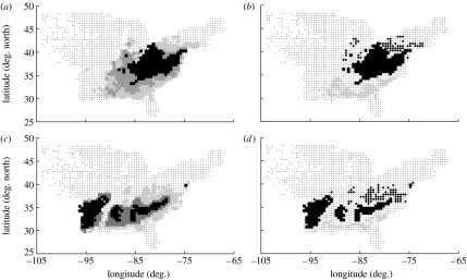
Figure 1.

(a,c) The range of each species was divided into three abundance bands according to the average abundance within 0.5×0.5° grid cells (see §2 and the electronic supplementary material). Cells not containing the species were omitted. Abundance band 0 (the third of cells with the greatest abundance; black squares) constitutes the core of the range; band 2 (the third of cell with the lowest abundance; light grey squares) constitutes the boundary of the range (abundance band 1, dark grey squares). (b,d) The northern boundary (diamonds) of the range consists of all cells within abundance band 2, and within the northernmost third of the cells occupied by the species; similarly, the southern boundary (circles) consists of all cells within abundance band 2, and within the northernmost third of the cells (squares, core). The crosses show all grid cells containing at least one forest inventory plot. Two example species are shown: (a,b) tulip tree (Liriodendron tulipifera) has a unimodal core (i.e. the core is contiguous), and a relatively symmetric range; (c,d) shortleaf pine (Pinus echinata) has a multimodal core and an asymmetric range.