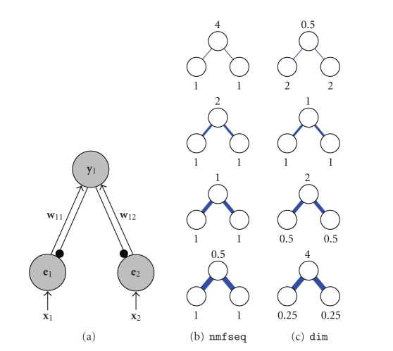
Figure 2.
(a) A simple neural network of the type used by all the algorithms described in this article (the symbols are the same as those used in Figure 1). This network has one output node which receives equal strength weights from two error-detecting nodes (i.e., w 11 = w 12). Each error-detecting node receives equal strength input from two-image pixels (i.e., x 1 = x 2 = 1). Each subfigure in (b) and (c) shows the steady-state activation strength of the output node and the two error-detecting nodes in this simple network calculated using (b) the sequential NMF algorithm, and (c) the divisive input modulation algorithm. The steady-state responses are calculated for different weight values (indicated by the width of each connection which is proportional to its strength). From top to bottom in (b) and (c) the weights (i.e., w 11 and w 12) are equal to 0.25, 0.5, 1, and 2. Note that there is no stochastic element in the calculation of the neural responses generated by these algorithms, so identical results will be generated each time the network is simulated with these weight values.

