
FIG. 2.
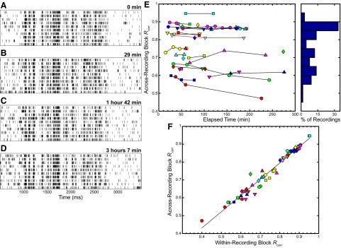
Illustration of spike-correlation–based similarity (Rcorr) over time. A–D: raster plots from the site whose STRFs are depicted in Fig. 1, A–D; time stamps at the top right corner of each raster plot indicate the time elapsed after the start of the 1st recording block obtained at the same site. E: plot of across-recording block Rcorr, where Rcorr was calculated between the responses from the 1st recording block and the responses from each subsequent recording block at a particular site plotted against the time elapsed after the start of the 1st recording block obtained at each site. To the right, a histogram shows the same data in bins of size 0.05. F: comparison of within-recording block Rcorr to across-recording block Rcorr, with a best-fit line plotted in black. The correlation coefficients was 0.98 (P < 0.001). In panels (E) and (F), the values of Rcorr for the data shown in (A–D) are outlined in red.