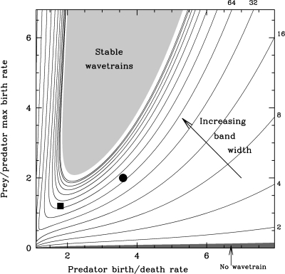
Fig. 6.

A contour plot of wavetrain band width as a function of parameters for the Rosenzweig–MacArthur predator–prey model (Eqs. 4). The contour levels have a power law spacing, with band width coefficient 𝒲 = 2,4,6,16,…,8192. The light shaded region corresponds to stable wavetrains behind invasion, and there is no wavetrain band for parameters in the shaded region immediately above the horizontal axis; in such cases, irregular oscillations develop immediately behind the invasion front. Two specific predator–prey systems are discussed in Example of Application: Predator–Prey Invasion, and the corresponding parameters are indicated in the figure by the square [weasels/field voles: a/b = 1.8, r/a = 1.2 (35)] and circle [zooplankton/phytoplankton: a/b = 3.6, r/a = 2.0 (43)]. The band width coefficients are calculated for c _inv = 2, because it is the “pulled” invasive front that is relevant in applications such as this (4, 33).