Figure 3. Screenshot of MSI Tomography’s database web interface tool.

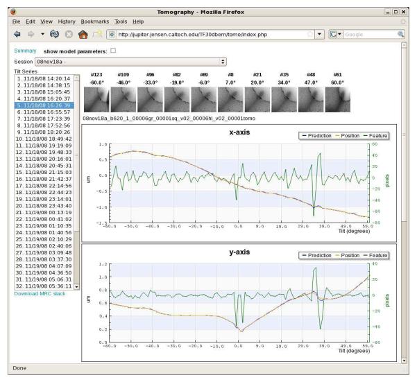
This tool allows users to review previous tilt series or check on the progress of current sessions from any web browser with access to the Leginon webserver. A drop-down list at the top allows the user to select the data collection session of interest (here “08nov18a”). The various tilt series collected during that session then appear as a list on the left. After a specific tilt series is selected (here “11/18/08 16:26:39”), a row of thumbnail images display snapshots of the tilt series at intervals throughout the tilt range to give the observer a visual sense of the target and how well it was tracked. Here, the target was a slender bacterial cell (long grey streak emerging from the bottom left corner of the images) whose tip is suspended over a circular hole in the carbon film. The movement of the specimen and the performance of the tracking algorithm are plotted below the thumbnails. Graphs for z height and image mean value also appear lower on the web page, but are not shown here for lack of space. Links to download an assembled MRC-format image stack (“Download MRC stack”) and display additional graphs of the energy slit and beam intensity change (“Summary”) are also provided.

In the plots, the green “feature” curves show how far away from the center of each image the target appeared (i.e. the tracking errors, in pixels, right vertical axes). The blue “prediction” curves report where the specimen was expected to be within the column as each image was taken, saved during the tilt-series as the total beam shift applied (in microns, left vertical axes). The orange “position” curves show the actual trajectory the specimen traversed (the sum of the beam shifts applied before the image was taken and the actual location of the target observed in the image, in microns, left vertical axes). The x-axes correspond to the tilt angle in degrees. Because the stage is physically re-centered on the target between the first and second halves of the tilt-series and two “untilted” images are recorded, there are actually two “0 plotted next to each other in the center.

In order to understand the relationship of the curves and the order of calculations and events, details of the first few operations shown will be described with reference to the “y-axis” plot, since the changes are large enough there to be followed in the graph. Before the tilt-series is acquired, the target is approximately centered on the CCD using stage shifts. The remaining fine shift needed to precisely re-center the target is done with beam shifts, and that shift is plotted as the first “prediction” point at 0 tilt. In this case the initial beam shift applied in the y-direction was 0.17 microns (blue curve, rightmost of the two adjacent 0° points). This value was considered the “actual” starting position of the specimen in the column as well, so the orange “position” curve begins at the same point. In the first image, the target was assumed to be correctly centered, so the green “feature” curve begins at exactly zero. Before the second image was taken, no predictions were made about how the specimen would move, so no additional beam shifts were applied, and the prediction curve for the 1° image remains flat at 0.17 microns. After the second image was recorded the position of the specimen in the image was measured by cross-correlation, and its deviation from the center (33 pixels) was plotted as the first tracking error (“feature” curve at 1°). The actual specimen position curve was therefore plotted an equivalent distance (0.03 microns) higher (note sign conventions are such that beam shift corrections oppose observed shifts in the images), at 0.2 microns. Given this first shift, a prediction was then made about where the specimen would be after the grid was tilted to 2°. The result was applied as a (modified) beam shift and plotted as the “prediction” (0.22 microns). This prediction proved largely correct, as the target then appeared just 2 pixels above the center of the 2° image (green curve). As a result, the “position” was also plotted as 0.22 microns (orange curve, 2°). Based on this trend, a further beam shift of 0.03 microns was applied before the 3° image was taken (blue curve now at 0.25, 3°), and so forth until the 60° image. The specimen can be seen to have moved quite steadily "up" in they direction, leading to very small tracking errors, until it unexpectedly hooked “down” between 34° and 39°, leading to tracking errors of first 30 pixels in one direction (34° and 35° images) and then 42 pixels in the other (37° image) before the tracking re-stabilized. After the first half of the tilt series was finished, the stage was rotated back to 0° and the target was roughly recentered with stage shifts. The remaining fine shifts needed to precisely recenter the target before the second half of the tilt series appear as the initial beam shifts (0.22 microns, blue and orange curves, leftmost 0° point). Only very slight tracking errors were seen in the second half of the tilt series (negative tilt angles).