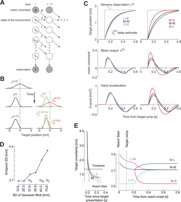
Figure 2.

The computational problem of estimating the state of the environment despite delay and noise in the sensory measurements. A, A “graphical model” representation of the delay and noise problems. Each circle depicts a random variable. The shaded circles are variables that are observed, and the unshaded circles are unobserved variables that must be estimated. The arrows describe conditional probabilities, or simply causality. The vector x represents information about state of the hand (position and velocity) and the target (its center). Observation y(t) is a measure of the delayed state xΔ(t). Given this observation, we need to estimate the current state x0(t) and then produce motor commands u such that the hand arrives in the center of the target. B, A simplified example of the estimation problem. The observation suddenly changes at time t. xΔ(t|t − δ) is the prior estimate before observation y(t) and x̂Δ(t|t) is the posterior estimate after the observation. With repeated observations, the mean of the estimate converges onto the observation. C, Simulations of a point mass system controlled by a time-delayed controller. Top row, The target jumps at t = 0. This change is observed after a time delay Δ = 100 ms. After the system observes the change in the target position, the estimated target position gradually converges to the observed target position. However, the speed of the convergence is affected by both the uncertainty of the prior (position of the target before it jumped) and the uncertainty of the observation (position of the target after it jumped). If the first target had a small uncertainty with respect to the second uncertainty, then the convergence rate is slow (e.g., S–M condition or M–L condition). If the first target had a large uncertainty with respect to the second uncertainty, then the convergence rate is fast (L–M and M–S conditions). Middle row, The motor command in response to the target jump. The peak response to the target jump is highest for L–M and M–S conditions. The duration of the response (time at which the curve crosses 0) is smallest for the L–M and M–S conditions. Bottom row, Motion of the simulated hand in response to the target jump. The peak response is higher and earlier in the L–M and M–S conditions. D, The endpoint SD of the simulated trajectories (500 trials in each condition). E, The time evolution of target uncertainty. Left, The uncertainty during the reaction time. Before the first target is displayed, uncertainty is very large. When the first target is displayed, the rate of reduction in the uncertainty is faster for the S target than for M or L targets. If we suppose that the system starts to initiate a reach a constant time after the uncertainty crosses an arbitrary threshold, then reaction times are shorter for S targets than for M or L. Right, The uncertainty during the reach when the target changes. By the time the reach starts, target uncertainty is near asymptotic levels. The uncertainty increases or decreases when the target changes. In the L–M condition, the uncertainty is higher than in the M–M or S–M conditions after the target jump, resulting in a greater reliance in the delayed sensory observations and therefore a faster correction.
