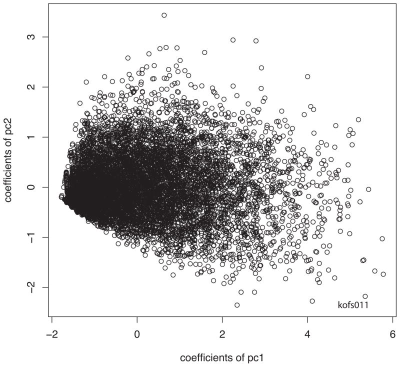
Figure 6.
Coefficients of second principal component vs coefficients of first principal component for each stimulus presentation. The narrow distribution at the left is a consequence of the spike trains being point processes. Because the first principal component is nearly the spike count, the number of spikes available for patterns of activity increases from left to right, so the number of patterns possible is small for low spike counts (left side of plot). Then numbers of spike patterns represented by the second principal component increase quickly with the increasing spike count, making for the cone-like structure in this plot. This shows that even though the principal components are orthogonal, they are not independent; higher coefficients of the first principal component lead to a larger range of values for the second.

