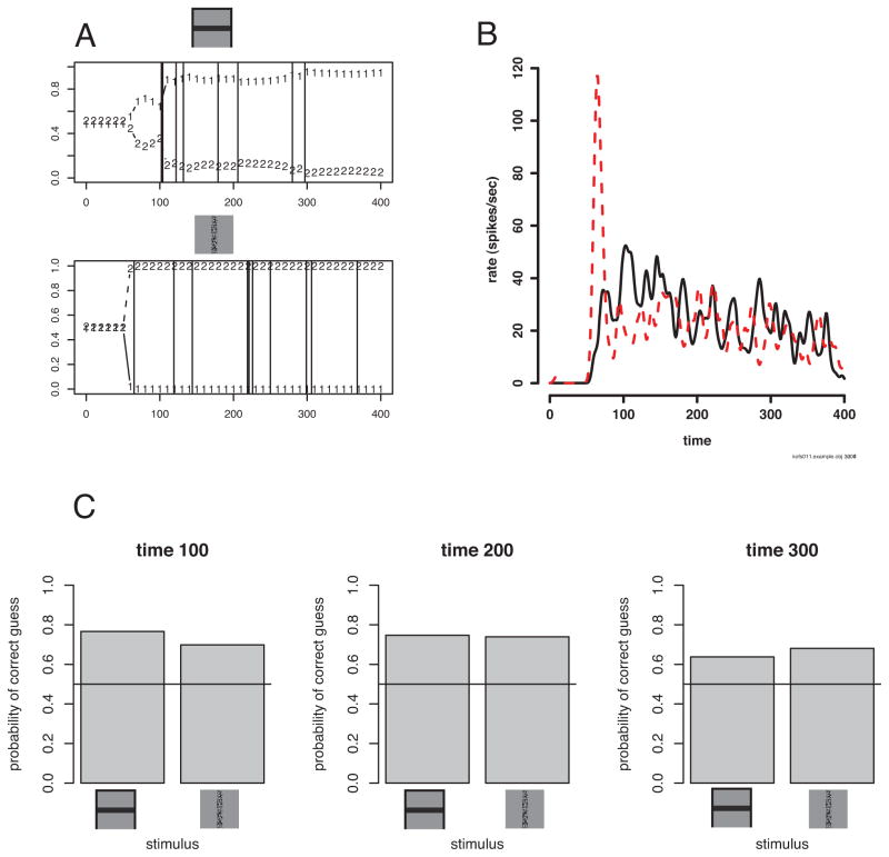
Figure 8.

Decoding of example from Figure 2. A. Millisecond-by-millisecond decoding for two spike trains with spike times shown as vertical lines. Because there are two stimuli in this example, the probability for random guessing is 0.5. B. The overlaid spike densities from Figure 2. The dashed line is the spike density for the speckled vertical bar and the solid line is for the horizontal black bar. This helps to explain the decoding, which starts before a spike for the black bar, because the decoder knows that if no spike has occurred by this time, the black bar is more likely. The value of the decoder is that it points to this feature of the spike densities. C. The decoding performance over the approximately 50 trials with each stimulus. The decoding accuracy does not improve after 100 ms for this example.