Spatial and temporal reproducibility-based ranking of the independent components of BOLD fMRI data

Abstract

Independent component analysis (ICA) decomposes fMRI data into spatially independent maps and their corresponding time courses. However, distinguishing the neurobiologically and biophysically reasonable components from those representing noise and artifacts is not trivial. We present a simple method for the ranking of independent components, by assessing the resemblance between components estimated from all the data, and components estimated from only the odd– (or even–) numbered time points. We show that the meaningful independent components of fMRI data resemble independent components estimated from downsampled data, and thus tend to be highly ranked by the method.

Introduction

Unlike positron emission tomography (PET), where a single image can report on brain blood flow, in blood oxygenation level dependent (BOLD) fMRI, functional information is contained only in the (often small) temporal modulation of the signal during the experimental paradigm. The acquired data are reduced to yield the familiar “activation maps,” most often using univariate inferential approaches, which test the same set of a priori temporal hypotheses in each image volume element (voxel). Statistical Parametric Mapping (Friston et al., 1995) employs the General Linear Model (GLM). Regression (using experimenter-defined time courses to model expected signal changes) allocates the temporal variance in the data among these time courses, followed by statistical inference thereby answering “where in the brain does the fMRI signal timing resemble the paradigm timing?”

Independent component analysis (ICA) ( -McKeown et al., 1998a,b) shares with the GLM the goal of expressing fMRI data as a sum of products of maps and time courses. Unlike GLM, ICA does not require the time courses to be specified in advance; rather an algorithm is used to find independent spatial maps and their associated time courses. However, interpretation of the resulting components – in particular, distinguishing meaningful (i.e., neurobiologically and biophysically reasonable) components from noise and artifacts – is not trivial. The need to examine all components is not helped by the fact that most ICA algorithms do not automatically rank the components by their relative importance. Ranking the components, for example, by percent variance is not generally helpful since nuisance sources of variance are often larger than the desired signals. Thus, this ranking issue has become an important challenge in the field of fMRI data analysis. While component assessment was initially performed by comparing maps to neuronatomical regions of interest, and time courses to paradigm timing, several groups have developed more sophisticated approaches for component assessment, such as power spectrum ranking (Moritz, Rogers, and Meyerand, 2003), support vector machine classifier (De Martino et al., 2007) and multiple (repeated) ICA estimations (Meinecke et al., 2000, Duann et al., 2003, Himberg, Hyvarinen, & Esposito, 2004, Yang, et al. 2008).

To test the reliability of consistently task-related (CTR) components estimated from fMRI data, McKeown et al. showed that an odd time-point and an even time-point data downsampling each yielded a component with a time course and map distribution resembling those of the original CTR component (McKeown et al, 1998b). Based on this report, we hypothesized that all meaningful components would be relatively highly reproducible, while many nuisance sources would tend to have poor reproducibility (except for some nuisance sources which would be stable across such decompositions, such as motion related and physiological pulsation related artifacts). Hence, we developed a simple approach that we call Maximum Mean Correlation, which ranks components by assessing resemblance between components estimated from all the data, and those estimated from downsampled data – specifically, from only the odd-numbered time points.

For each data set, two separate ICA estimations are performed: One (“ALL”) on all the data, and one (“ODD”) on only the odd time point data. Temporal and spatial correlations are computed between each ALL component and each ODD component; the average of the temporal and spatial correlation is defined as the mean correlation. The maximum mean correlation (MMC) for each ALL component, with respect to the set of ODD components, is used to sort the ALL components. A second MMC ranking is performed using the even time point data; the ODD and EVEN downsamplings provide a consistency check of the MMC rankings.

Thus, using our MMC approach, the independent components of BOLD fMRI data are ranked according to how well each one resembles any of the components estimated from downsampled data. Results show that this procedure generally ranks meaningful components high, and less meaningful components low.

Methods

Data Acquisition

Five adults (two male) gave informed consent to participate in IRB-approved research. Data were acquired on a Philips 3.0 Tesla scanner using a multi-element receiver coil to allow partially parallel image acquisition. BOLD fMRI data were acquired using single-shot SENSE gradient echo EPI with 37 slices providing whole-brain coverage, a SENSE acceleration factor of 2.0, a TR of 2.0 s and scan resolution of 80 × 80. Nominal in-plane resolution was 3mm × 3mm; slice thickness was 3 mm; slice gap was 1 mm.

Participants underwent four fMRI scans, each of 4 minute duration with 120 time points: one while they rested quietly with their eyes closed, and three using as visual stimulus a radial blue/yellow checkerboard, reversing at (nominal) 7 Hz, presented using three different paradigm timings. The three visual paradigms were: block design (20 s on, 20 s off); slow event-related (2 s on; 12 s off); rapid jittered event-related (2 s on; mean stimulus onset asynchrony (SOA) 6 s). The order of the four conditions was counterbalanced across sessions. The resting data was used to create “hybrid” data by adding simulated signals; this method is described below.

Hybrid Data

To assess MMC performance at finding known sources, two simulated signals were added, at an amplitude equal to 0.05 times the average amplitude of the signal within the brain. Figure 1A displays the spatial maps. The signal change in the anterior two regions and the more posterior two regions respectively correspond to mixing function 1 and mixing function 2, as shown in Figure 1 B.

Figure 1.

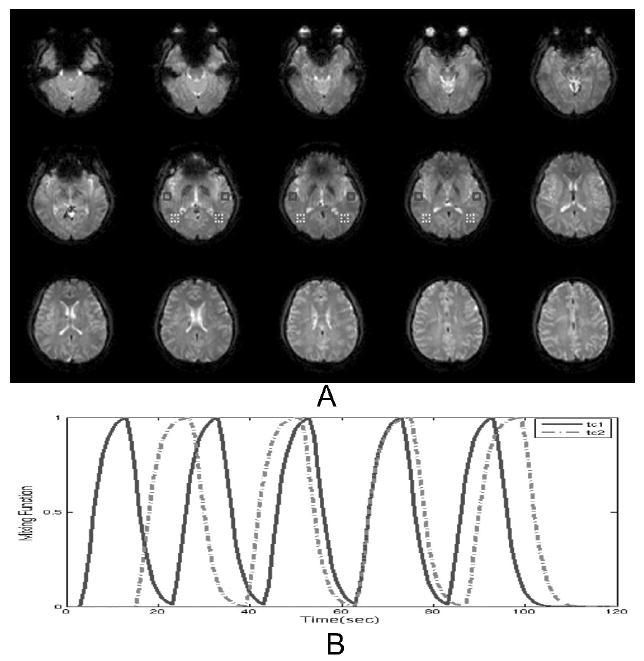
A. Hybrid data: Echo planar images from resting participant; red boxes indicate where the simulated signals are added. The simulated signals refer to change in the anterior two regions and the more posterior two regions respectively. B. Time courses for the two simulated sources. They are generated by using a gamma variate function for the hemodynamic response function with delay 1.3 in the function.

Independent Component Analysis

Preprocessing was accomplished using the FSL (FMRIB’s Software Library, www.fmrib.ox.ac.uk/fsl) software package (Smith et al., 2004) which included removal of non-brain voxels; voxel-wise de-meaning; normalization of voxel-wise variance; slice-timing correction; motion correction; temporal high-pass filtering; and spatial smoothing using a Gaussian kernel with a full-width at half-maximum (FWHM) of 8mm. ICA, including automatic estimation of dimensionality by probabilistic principal component analysis (PPCA), was performed using MELODIC v. 2.0 (Multivariate Exploratory Linear Decomposition into Independent Components) (Beckmann and Smith 2004), which is part of FSL. ICA decomposition yields spatial maps and their associated time courses; maps are thresholded using MELODIC’s default threshold of 0.5, a value that assigns equal ‘cost’ to false-positives and false-negatives when determining the probability that a voxel is classified as part of a component rather than as noise.

Maximum Mean Correlation

For each study, separate ICA estimations were performed on the entire data set, and on its subsampled data. We refer to components estimated from the full data as ALL components, and to components estimated from the odd time point data as ODD components. The time courses of the ALL components were subsampled to allow comparison with time courses of the ODD components. Spatial (equation 1) and temporal (equation 2) absolute correlation coefficients were computed between each ALL component and each ODD component:

$$\begin{array}{l}{r}_s=\mathit{abs}\left(\frac{\sum _m\sum _n\sum _k\left(S_{1_{\mathit{mnk}}}-\overline{S_1}\right)\left(S_{2_{\mathit{mnk}}}-\overline{S_2}\right)}{\sqrt{\left(\sum _m\sum _n\sum _k{\left(S_{1_{\mathit{mnk}}}-\overline{S_1}\right)}^2\right)\left(\sum _m\sum _n\sum _k{\left(S_{2_{\mathit{mnk}}}-\overline{S_2}\right)}^2\right)}}\right)\\ m=1,2,\dots ,M-1,M;n=1,2,\dots ,N-1,N;k=1,2,\dots ,K-1,K\end{array}$$ (1)

where S₁, S₂ represent the unthresholded spatial statistic maps with dimensions M × N × K; $\overline{S_1}$, $\overline{S_2}$ are their respective three-dimensional mean values; r_S is the absolute spatial correlation coefficient. We define

$$\begin{array}{c}{r}_T=\mathit{abs}\left(\frac{\sum _i\left(A_{1_i}-\overline{A_1}\right)\left(A_{2_i}-\overline{A_2}\right)}{\sqrt{\left(\sum _i{\left(A_{1_i}-\overline{A_1}\right)}^2\right)\left(\sum _i{\left(A_{2_i}-\overline{A_2}\right)}^2\right)}}\right)\\ i=1,2,\dots ,I-1,I\end{array}$$ (2)

where A₁, A₂ represent the compared temporal time courses with I points; $\overline{A_1}$, $\overline{A_2}$ are their respective mean values; r_T is the absolute temporal correlation coefficient.

Presumably meaningful IC components tend to have high spatial reproducibility and high temporal reproducibility, hence in our approach, spatial and temporal absolute correlation coefficients were then averaged to yield the mean correlation r̄.

For each ALL component, the maximum value of r̄ was calculated with respect to the set of ODD components:

$${\mathit{MMC}}_i=\underset{j}{\mathit{MAX}}({\overline{r}}_{\mathit{ij}})$$ (3)

Here MMC_i refers to the Maximum Mean Correlation of the i th component from the ALL data; r̄_ij is the mean correlation coefficient between the i th component of the ALL data and the j th component of the downsampled data, in this case the ODD components. Components were then ordered using MMC_i as each component’s ranking score.

In addition, the MMC ranking procedure was performed again on data that was downsampled from the even time point data. Thus, two MMC rankings are obtained using downsampled data, one based on the odd time points, and one based on the even time points. Comparing these rankings yields a consistency measure for the MMC rankings.

Group Analyses

Data for each paradigm were entered into group Independent Component Analyses using the multi-session temporal concatenation approach in MELODIC Version 3.05. Group ICA estimations were performed on the data for each paradigm, and on their respective downsampled odd- and even-numbered time point data; MMC was used to rank the resulting group components.

Inferential Analyses

As a check on the exploratory analyses performed using ICA, inferential analysis using the General Linear Model as implemented in FEAT (FMRI Expert Analysis Tool, http://www.fmrib.ox.ac.uk/analysis/research/feat/) Version 5.1, part of the FSL software library, was performed on the hybrid data, and on data from each visual paradigm. This GLM analysis yielded Z statistic maps, thresholded at Z>2.3, and their associated full model fitting time courses.

Spatial correlation coefficients were calculated between the GLM thresholded z-map and each MMC ranked component thresholded spatial map. Similarly, temporal correlation coefficients were computed between the GLM time course and each MMC ranked component time course.

Furthermore, group ICA results were compared to GLM mixed-effects group analysis results as generated by FLAME (FMRIB’s Local Analysis of Mixed Effects; Woolrich et al., 2003).

Comparison with other Ranking Approaches

To compare MMC ranking with other ranking approaches, simulated signals were added to specific regions in the resting data, at varying contrast to noise (CNR) levels.

MMC ranking was compared with five other ranking approaches, namely percent variance (McKeown et al., 1998); multi parameter ranking based on spatial clustering and one-lag serial autocorrelation (Formisano, et al, 2002); ranking based on the one-lag spatial serial autocorrelation; one-lag temporal autocorrelation; the average of one-lag temporal and one-lag spatial autocorrelations; and the power spectrum method, which requires knowledge of source frequency (Moritz, Rogers, and Meyerand, 2003). For this purpose, one known source was added, to yield contrast-to-noise ratios of 0.5 to 0.65, 0.8, and 0.95. For each CNR level, eight realizations were respectively constructed. Figure 2 shows the mixing functions and one mixing region.

Figure 2.

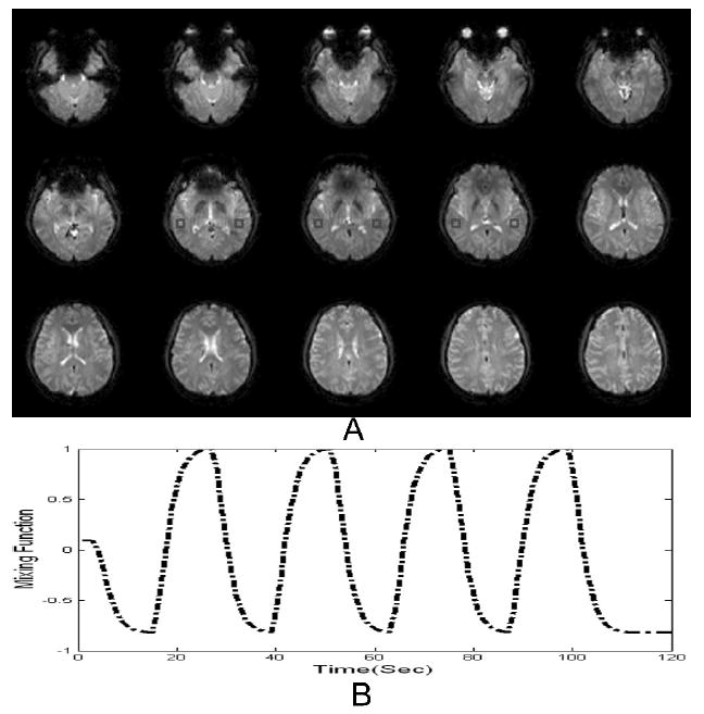
Hybrid data for testing different ranking methods at each Contrast to Noise Ratio (CNR): A. Red boxes indicate where the simulated signals are added; B. Mixing function for the simulated sources.

For this analysis, ICA decomposition was performed using MELODIC, with the number of components set to 40 for both ALL and subsampled data sets. For each of the eight realizations at each of the 4 CNR levels, independent components were estimated and then ranked using MMC and the six other approaches.

Results

Hybrid data

ICA of representative hybrid data yielded 23 components; ICA of its odd-downsampled data and even-downsampled data respectively yielded 17 components and 19 components. Figure 3 displays the consistency of MMC ranking using odd and even downsampling. The two rankings were highly correlated with a correlation coefficient of 0.80 and a p-value < 0.005. MMC-ranked maps and time courses (with respect to the set of ODD components) are shown in Figure 4. GLM analysis results are also displayed in the last two panels (GLM_1 and GLM_2) in the figure. The GLM_1 map has high spatial correlation of 0.92 with the first (labeled #1) MMC-ranked component map and has low spatial correlation of less than 0.1 with any other component map. The GLM_1 time course has high temporal correlation of 0.81 with the first MMC-ranked component time course and has low temporal correlation of less than 0.26 with any other component time course; the GLM_2 map has high spatial correlation of 0.89 with the second (labeled #2) MMC-ranked component map and has low spatial correlation of less than 0.1 with any other component map; the GLM_2 time course has high temporal correlation of 0.86 with the second MMC-ranked component time course and has low temporal correlation of less than 0.2 with any other component time course. Results are summarized in Table 1.

Figure 3.

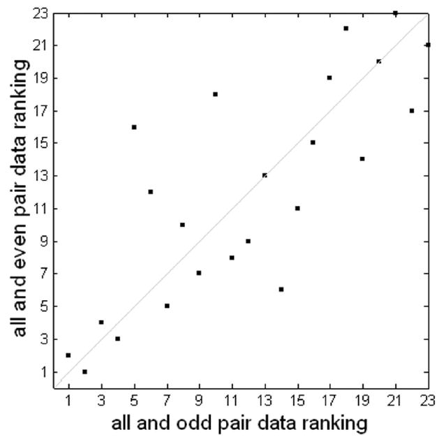
Consistency of MMC ranking of hybrid data using odd and even downsampling. The two rankings have a correlation coefficient of 0.80 and a p-value < 0.005.

Figure 4.

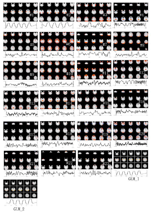
MMC ranked components from hybrid data, with GLM analysis results (last two panels). The top-ranked two components capture the simulated sources. To save space, not all slices are shown.

Table 1.

Temporal and spatial correlation coefficients between MMC ranked components and GLM results for hybrid data (Hybrid), block design visual paradigm data (Block), slow event-related visual paradigm data (Slow), jittered event-related visual paradigm data (Jittered) and group jittered event-related paradigm data (Group).

Data	MMC ranking	Corr. between MMC ranking and GLM results (Temporal/Spatial)
Hybrid	#1	0.81 / 0.92
	#2	0.86 / 0.89
	Remaining rankings	< 0.26 / < 0.10
Block	#1	0.96 / 0.92
	Remaining rankings	< 0.27 / < 0.20
Slow	#1	0.80 / 0.85
	Remaining rankings	< 0.29 / < 0.25
Jittered	#1	0.66 / 0.87
	Remaining rankings	< 0.14 / < 0.06
Group	#1	0.95 / 0.94
	Remaining rankings	< 0.54 / <0.38

Block design visual paradigm

ICA of representative data from the simple block-design visual paradigm yielded 19 components; ICA of its odd-downsampled data and even-downsampled data respectively yielded 16 components and 15 components. Figure 5 shows the consistency of MMC ranking using odd and even downsampling. The two MMC rankings were significantly consistent with a correlation coefficient of 0.68 and a p-value < 0.005. The maps and time courses of the MMC ranked components (with respect to the set of ODD components) are shown in Figure 6. GLM analysis results are also included in the last panel (GLM_1) in the figure. Table 1 displays temporal and spatial correlation coefficients between MMC-ranked components and GLM results. The GLM_1 map has high spatial correlation of 0.92 with the first MMC-ranked component map and has low spatial correlation of less than 0.20 with any other component map; the GLM_1 time course has high temporal correlation of 0.96 with the first MMC-ranked component time course and has low temporal correlation of less than 0.27 with any other component time course.

Figure 5.

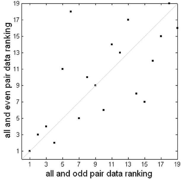
Consistency of MMC ranking of block-design using odd and even downsampling. The two rankings have a correlation coefficient of 0.68 and a p-value < 0.005.

Figure 6.

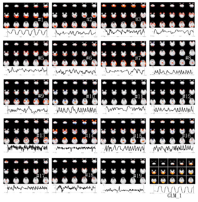
Ranked components from simple block-designed visual paradigm, with GLM analysis results (last panel). The first component captures the response to the visual stimuli in primary visual cortex. To save space, not all slices are shown.

Slow event-related visual paradigm

ICA of representative data from the slow event-related visual paradigm yielded 23 components; ICA of its odd-downsampled data and even-downsampled data respectively yielded 19 components and 18 components. Figure 7 shows the consistency of MMC ranking using odd and even downsampling. The two MMC rankings were significantly consistent with a correlation coefficient of 0.67 and a p-value < 0.005. The maps and time courses of the MMC ranked components (with respect to the set of ODD components) are shown in Figure 8. GLM analysis results are also shown in the last panel (GLM-1) in the figure. The GLM_1 map has high spatial correlation of 0.85 with the first MMC-ranked component map and has low spatial correlation of less than 0.25 with any other component map; the GLM_1 time course has high temporal correlation of 0.80 with the first MMC-ranked component time course and has low temporal correlation of less than 0.29 with any other component time course. These temporal and spatial correlation coefficients are shown in Table 1.

Figure 7.

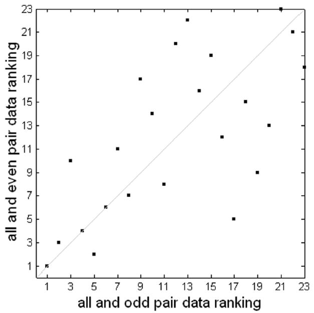
Consistency of MMC ranking of slow even-related data using odd and even downsampling. The two rankings have a correlation coefficient of 0.67 and a p-value < 0.005.

Figure 8.

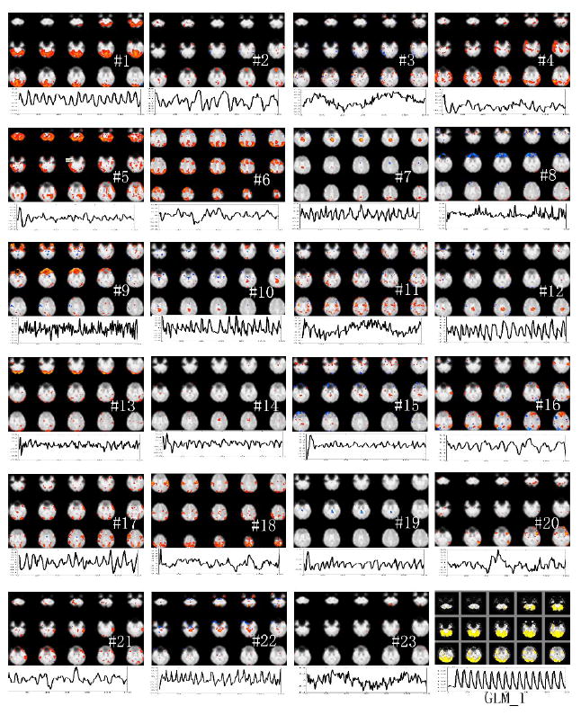
Ranked components from slow event-related paradigm, and GLM analysis results (last panel). The first component captures the response to the visual stimuli in primary visual cortex. To save space, not all slices are shown.

Jittered event-related visual paradigm

ICA of representative data from the jittered event-related visual paradigm yielded 21 components; ICA of its odd-downsampled data and even-downsampled data respectively yielded 14 components and 15 components. Figure 9 shows the consistency of MMC ranking using odd and even downsampling. The two MMC rankings were significantly consistent with a correlation coefficient of 0.56 and a p-value < 0.005. The maps and time courses of the MMC ranked components (with respect to the set of ODD components) are shown in Figure 10. GLM analysis results are also included in the last panel (GLM_1) in the figure. Table 1 displays temporal and spatial correlation coefficients between the MMC ranked components and GLM results, where the GLM_1 map has high spatial correlation of 0.87 with the first MMC-ranked component map and has low spatial correlation of less than 0.06 with any other component map; the GLM_1 time course has high temporal correlation of 0.66 with the first MMC-ranked component time course and has low temporal correlation of less than 0.14 with any other component time course.

Figure 9.

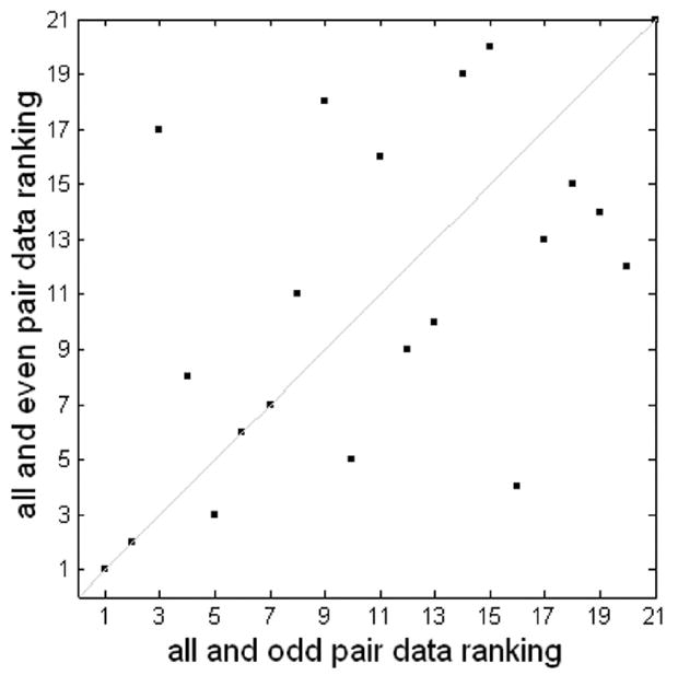
Consistency of MMC ranking of rapid jittered-related data using odd and even downsampling. The two rankings have a correlation coefficient of 0.56 and a p-value < 0.005.

Figure 10.

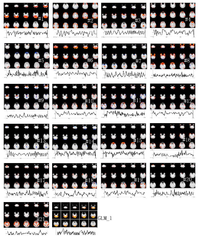
Ranked components from jittered event-related paradigm, with GLM analysis results (last panel). The first component captures the response to the visual stimuli in primary visual cortex. To save space, not all slices are shown.

Group Analyses

Group ICA of data from the block design paradigm, the slow event-related visual paradigm, and the jittered event-related visual paradigm yielded 26, 26, and 25 components, respectively. ICA of their odd-downsampled data respectively yielded 24, 26, and 21 components, and ICA of their even-downsampled data respectively yielded 23, 25, and 21 components. Group ICA results for the jittered event-related data are displayed in Figures 11 and 12. Figure 11 shows the consistency of MMC ranking using odd and even downsampling. The two MMC rankings were significantly consistent with a correlation coefficient of 0.66 and a p-value < 0.005. The maps and time courses of the MMC ranked components (with respect to the set of ODD components) are shown in Figure 12. GLM analysis results are also included in the last panel (GLM_1) in the figure. Table 1 displays temporal and spatial correlation coefficients between the MMC ranked components and GLM results, where the GLM_1 map has high spatial correlation of 0.94 with the first MMC-ranked component map and has low spatial correlation of less than 0.38 with any other component map; the GLM_1 time course has high temporal correlation of 0.95 with the first MMC-ranked component time course and has low temporal correlation of less than 0.54 with any other component time course.

Figure 11.

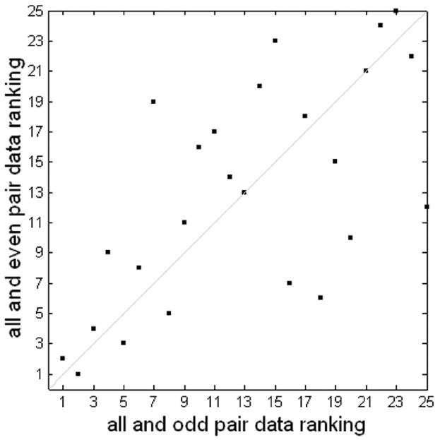
Consistency of MMC ranking of group jittered event-related data using odd and even downsampling of the group data. The two rankings have a correlation coefficient of 0.66 and a p-value < 0.005.

Figure 12.

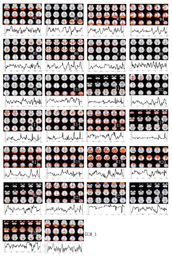
Ranked components from group jittered paradigm event-related data, with GLM results (final panel). The first component captures the response to the visual stimuli in primary visual cortex. To save space, not all slices are shown.

Comparison with Other Ranking Methods

Simulated activation data, created by adding a known signal to resting state data at four CNR levels, were analyzed using ICA and the resulting components ranked using MMC and six other ranking approaches. Figure 14 shows the ranking order (i.e., “1” means first-ranked component) of the component capturing the known source for each ranking method, as a function of CNR, averaged over the eight realizations of each CNR value. Here, ‘MMC’, ‘MPR’, ‘TEMP’,’SPAT’,’MIX’, ‘VAR’ and ‘POWER’ respectively represent maximum mean correlation (MMC), multi parameter ranking (MPR) and ranking based on one-lag temporal autocorrelation (TEMP), one-lag spatial autocorrelation (SPAT), average values of one-lag temporal and one-lag spatial autocorrelation (MIX), percent variance (VAR) and the power spectrum ranking (POWER). All methods performed well at the highest CNR studied, while performance differed at low CNR (see discussion).

Figure 14.

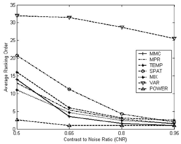
The average ranking of the component capturing the known source vs. contrast-to-noise ratio for six ranking approaches: ‘MMC’ = maximum mean correlation; ‘MPR’ = multi parameter ranking; ‘TEMP’ = one-lag temporal autocorrelation, ‘SPAT’ = one-lag spatial autocorrelation, ‘MIX’ = average of one-lag temporal and one-lag spatial autocorrelation; ‘VAR’ = percent variance, ‘POWER’ = power spectrum.

Discussion

In this study, fMRI data reporting on block and event-related design were acquired and their independent components were calculated. Unlike most studies applying ICA to fMRI data, this study illustrates all the estimated independent components, not just those judged most relevant to task or a priori brain regions of interest. As most ICA algorithms present the components in no meaningful order, this study is focused on ordering them according to how well each one resembles any of the components estimated from downsampled data.

For the hybrid data (resting state plus two simulated sources), the two highest-ranked components capture the simulated sources, as they agree both in space and time with the simulated sources (Figure 4). The next eight highest-ranked components appear meaningful: the maps resemble familiar functional brain regions, such as primary visual (component 3) and auditory (component 9) cortex, and/or previously reported “resting state components” (Beckmann et al, 2005, Raichle et al., 2001). Additionally, these time courses contain power predominantly at low temporal frequencies consistent with hemodynamically-modulated BOLD signals. Conversely, the lowest-ranked components do not appear meaningful: their maps either depict widely distributed bi-phasic (“salt and pepper”) signals, or appear consistent with pulsation or bulk motion, and their time courses contain strong high-frequency signals consistent with noise and/or motion, but not with hemodynamically-modulated BOLD signals. For all data sets, the consistency of the odd- and even-based downsampling MMC rankings was excellent.

For the simple block-design visual paradigm, the component ranked highest by MMC evidently captures the BOLD fMRI signal response to the visual stimuli, as this component is primarily localized to early visual cortex, is synchronous with the stimulus timing, and agrees with the GLM analysis of these data (Figure 6).

For both the slow and the jittered event-related paradigms, the components ranked highest by MMC also evidently capture the BOLD fMRI signal response to the visual stimuli, and agree with the GLM analyses of their respective data (Figure 8; Figure 10).

For group ICA of the three sets of visual stimuli data, the component ranked highest in each case by MMC evidently captures the BOLD fMRI signal response to the visual stimuli, and agrees with the GLM analysis of their respective data.

For each analysis, the default PPCA used by MELODIC may estimate a different number of components from the whole data set and its associated temporally downsampled data. However, because all our results show that MMC ranks meaningful components very highly, we can conclude that temporal downsampling does not eliminate any of these meaningful sources. Furthermore, if we do not use PPCA to estimate the number of components in each decomposition, but instead force ICA of the downsampled data to yield the same number of components as for the full data, we find very little effect on the MMC rankings. For example, Figure 13 shows the consistency of MMC ranking for hybrid data decomposition with and without PPCA. Without PPCA, the number of components was fixed at 40 for decomposition of both the full and the odd-downsampled data; with PPCA, 23 components were estimated from the full data and 17 components were estimated from the odd-downsampled data. The two MMC rankings are consistent, with a correlation coefficient of 0.7352 and a p-value < 0.005.

Figure 13.

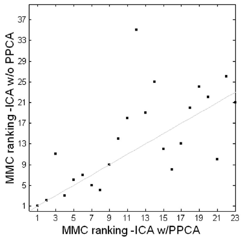
Consistency of MMC ranking for hybrid data decomposition with PPCA and without PPCA. The two MMC rankings have a correlation coefficient of 0.7352 and a p-value < 0.005.

Thus, using fMRI data from both block and event-related designs, and from both single subjects and groups, we have shown that the MMC approach may be generally useful for ranking the independent components of fMRI data.

The effectiveness of our approach appears to depend on the nature of the paradigm, as the temporal correlation between the first-ranked component and the GLM regressor decreases as the paradigm changes from block design to event-related, presumably because of the higher temporal frequency content of the signal from the more rapid paradigms.

The effectiveness of MMC ranking depends also on the contrast to noise ratio. Figure 14 shows excellent MMC performance at CNR = 0.95, and poorer performance as CNR decreases. Figure 14 also shows that MMC has better performance than the other five non-prior-knowledge ranking methods for intermediate CNR values. Figure 14 also shows power spectrum method has the best performance at most CNR levels. Thus if the source frequency is known, this approach may be best.

Our hypothesis was that MMC would be effective because meaningful components would be more reproducible, and hence robust with respect to downsampling, than artifactual components. However, some artifactual components are reproducible and robust, and so some artifactual components are highly-ranked by MMC. For example, Figure 15 shows eight selected highly ranked (by MMC) components estimated from resting state data. Components, 1, 2, 3, and 5 refer to meaningful components, while the others appear to be artifactual components. Among them, component No. 4 and component No. 20 correspond to abrupt motion; component No. 11 to CSF space pulsation; and component No. 33 to blood vessel pulsation. Table 2 shows the respective spatial correlations and temporal correlations between ALL data and the down-sampled (ODD) data. Due to its high spatial and temporal reproducibility, the parietal lobe motion artifact source was ranked fourth. Note that the posterior cingulate cortex (PCC) default mode source (Raichle, M. E. et. al. 2001) was ranked lower than this motion artifact, even though it has more spatial correlation. In addition, we found the meaningful components usually have both high temporal reproducibility and high spatial reproducibility, but most artifactual components tend to have lower spatial reproducibility, even if they also have high temporal reproducibility, such as components No. 20 and No. 33.

Figure 15.

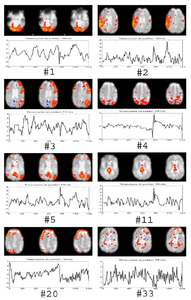
Selected MMC ranked components. # 1 means the first ranking component. See text for details.

Table 2.

Temporal and spatial correlation coefficients between ALL data and ODD data of eight selected MMC ranked components from a resting data set.

Component	No. 1	No. 2	No. 3	No. 4	No. 5	No. 11	No. 20	No. 33
Spat. Corr.	0.8257	0.7347	0.7267	0.7188	0.6832	0.5887	0.4358	0.2904
Temp. Corr.	0.8955	0.9313	0.8917	0.8665	0.8672	0.8746	0.6208	0.5089

While MMC appears to rank meaningful components above artifactual components, the rankings of meaningful components depend upon their strength. Therefore, neural correlates of e.g. primary sensory stimulation and motor responses may be ranked above neural correlates of the higher cognitive functions that may be the target of a study. For this reason, the MMC rankings should not be interpreted as indicative of any sort of absolute importance.

Relation to prior work

McKeown performed ICA separately on the odd and even time points of fMRI data, then used spatial correlation of the resulting maps to demonstrate reproducibility of the “consistently task related” component (McKeown, 1998b). Our approach takes advantage of such reproducibility by developing it into a ranking criterion for all components.

Repeated ICA decomposition has been used to assess the reproducibility of independent components. Meinecke et al., proposed a bootstrap resampling approach to determine reproducibility across decompositions (Meinecke et al., 2000). McKeown applied two sequential ICA estimations with different initial weight matrices, and reported highly reproducible components by comparing results from the two decompositions using mutual information (McKeown, 2002). Duann et al., assessed the consistency and stability of components obtained from mutiple infomax ICA decompositions (Duann et al., 2003).

Himberg et al., use a graphical approach to assess consistency between repeated ICA estimations performed on the same data (Himberg, Hyvarinen, & Esposito, 2004). The motivation for their work is that the iterative FastICA algorithm will yield different results depending on the starting or seed point, and so repeated estimations are valuable in assessing consistency of ICA results. This approach has recently been extended to other ICA algorithms (Correa, Adali, & Calhoun, 2007).

Yang et al., also utilized repeated ICA decomposition on the same data and then relied on the spatial reproducibility between them to order and select components (Yang, et al. 2008). In contrast, MMC ranks components based on the spatial and temporal resemblance of independent components extracted from the whole data set with independent components from the temporally downsampled data set.

Moritz et al., use a power spectrum ranking approach for identification of task-related components using the fundamental paradigm task frequency (Moritz, Rogers, and Meyerand, 2003). Our data show that it is the best-performing method at low CNR level. However, the MMC approach does not require information on paradigm timing.

McKeown proposed a hybrid ICA technique, HYBICA, which combines a data-driven ICA approach with a hypothesis-driven GLM approach, to separate consistently meaningful task-related components from non-relevant components (McKeown, 2000). In contrast, MMC does not require any specification of paradigm timing.

Further studies

The downsampling approach used for MMC ranking rejects signals at high temporal frequencies, but is not equivalent to a simple lowpass filter, nor is MMC ranking equivalent to a simple low-frequency weighting. For example, component number 9 in the hybrid data is the “slowest” component but is not ranked highest by MMC (see Figure 4). Other approaches to temporal-frequency based filtering and weighting may be worthy of exploration.

Here we have used only (deterministic) downsampling by a factor of two. Other downsampling ratios and schemes are possible. For example, we have found (not shown) that a factor of 1.5 is also effective for MMC ranking.

The effectiveness of MMC ranking presumably depends upon the relationship between the sampling frequency (or TR) and the temporal frequencies of the signals of interest. All data in this report were acquired using TR = 2 sec. In order to simulate data with slower sampling (longer TR), we applied downsampling to data from our block-design visual stimuli, to yield an effective TR = 4 s (downsampling by a factor of two) and 8 s (downsampling by a factor of four). Applying ICA and then MMC to these data (not shown) consistently ranked the main “visual component” as first. Further study is needed to test data with much slower sampling (very long TR), as is used for acquisitions employing sparse temporal sampling (Hall et al., 1999).

The effectiveness of MMC ranking also depends on the spatial extent of sources. We tested this by changing the size of one source region in our simulations. Preliminary results (not shown) show most simulated sources were ranked the highest at the four CNR levels, regardless of size.

Ranking components assists with, but does not solve completely, the problem of assessing which components matter. We note that Martino et al., applied support vector machine classifiers to “IC-fingerprints” for this purpose (De Martino et al., 2007).

Conclusion

We propose ranking the independent components of fMRI data according to their resemblance to components estimated from only the odd time point data. We have shown that this tends to rank the meaningful components high, presumably because the hemodynamic response underlying BOLD fMRI is slow relative to typical fMRI sampling rates (0.5 Hz, corresponding to a TR of 2 s), while most artifacts tend to have higher temporal and/or spatial frequency, and/or be less reproducible. This simple approach to the ranking of components from ICA of fMRI data is expected to have wide applicability.

References

- Beckmann CF, Smith SM. Probabilistic independent component analysis for functional magnetic resonance imaging. IEEE Trans on Medical Imaging. 2004;23(2):137–152. doi: 10.1109/TMI.2003.822821. [DOI] [PubMed] [Google Scholar]
- Beckmann CF, DeLuca M, Devlin JT, Smith SM. Investigations into resting-state connectivity using independent component analysis. Philos Trans R Soc Lond B Biol Sci. 2005;360(1457):1001–1013. doi: 10.1098/rstb.2005.1634. [DOI] [PMC free article] [PubMed] [Google Scholar]
- Correa N, Adali T, Calhoun VD. Performance of blind source separation algorithms for fMRI analysis using a group ICA method. Magn Reson Imaging. 2007;25(5):684–494. doi: 10.1016/j.mri.2006.10.017. [DOI] [PMC free article] [PubMed] [Google Scholar]
- De Martino F, Gentile F, Esposito F, Balsi M, Di Salle F, Goebel R, Formisano E. Classification of fMRI independent components using IC-fingerprints and support vector machine classifiers. Neuroimage. 2007;34(1):177–194. doi: 10.1016/j.neuroimage.2006.08.041. [DOI] [PubMed] [Google Scholar]
- Duann J-R, Jung T-P, Makeig S, Sejnowski TJ. Consistency of infomax ICA decomposition of functional brain imaging data. 4rd International Symposium on Independent Component Analysis and Blind Signal Separation; Nara, Japan. 2003. pp. 290–294. [Google Scholar]
- Friston KJ, Holmes AP, Poline JB, Grasby PJ, Williams SC, Frackowiak RS, Turner R. Analysis of fMRI time-series revisited. Neuroimage. 1995;2(1):45–53. doi: 10.1006/nimg.1995.1007. [DOI] [PubMed] [Google Scholar]
- Formisano E, Esposito F, kriegeskorte N, Tedesci G, Di Salle F, Goebel R. Spatial independent component analysis of functional magnetic resonance imaging time-series: characterization of the cortical components. Neurocomputing. 2002;49:241–254. [Google Scholar]
- Hall DA, Haggard MP, Akeroyd MA, Palmer AR, Summerfield AQ, Elliott MR, Gurney EM, Bowtell RW. “Sparse” temporal sampling in auditory fMRI. Hum Brain Mapp. 1999;7(3):213–223. doi: 10.1002/(SICI)1097-0193(1999)7:3<213::AID-HBM5>3.0.CO;2-N. [DOI] [PMC free article] [PubMed] [Google Scholar]
- Himberg J, Hyvarinen A, Esposito F. Validating the independent components of neuroimaging time series via clustering and visualization. Neuroimage. 2004;22(3):1214–1222. doi: 10.1016/j.neuroimage.2004.03.027. [DOI] [PubMed] [Google Scholar]
- McKeown MJ, Jung TP, Makeig S, Brown G, Kindermann SS, Lee TW, Sejnowski TJ. Spatially independent activity patterns in functional MRI data during the stroop color-naming task. Proc Natl Acad Sci. 1998a;95(3):803–810. doi: 10.1073/pnas.95.3.803. [DOI] [PMC free article] [PubMed] [Google Scholar]
- Mckeown MJ, Makeig S, Brown G, Jung T, Kindermann SS, Bell AJ, Sejnowski TJ. Analysis of fMRI data by bilind separation into independent spatial components. Human Brain Mapping. 1998b;6(3):160–188. doi: 10.1002/(SICI)1097-0193(1998)6:3<160::AID-HBM5>3.0.CO;2-1. [DOI] [PMC free article] [PubMed] [Google Scholar]
- McKeown MJ. Detection of consistently task-related activations in fMRI data with hybrid independent component analysis. NeuroImage. 2000;11(1):24–35. doi: 10.1006/nimg.1999.0518. [DOI] [PubMed] [Google Scholar]
- McKeown MJ. Deterministic and stochastic features of fMRI data: Implications for data averaging. In: Sommer FT, Wichert A, editors. Exploratory Analysis and Data Modeling in Functional Neuroimaging. The MIT Press; Cambridge, Massachusetts: 2002. pp. 63–76. [Google Scholar]
- Meinecke F, Ziehe A, Kawanabe M, Müller K-R. Assessing reliability of ICA projections - A resampling approach. 3rd International Symposium on Independent Component Analysis and Blind Signal Separation; San Diego. 2000. pp. 74–79. [Google Scholar]
- Moritz CH, Rogers BP, Meyerand ME. Power spectrum ranked independent component analysis of a periodic fMRI complex motor paradigm. Hum Brain Mapp. 2003;18(2):111–122. doi: 10.1002/hbm.10081. [DOI] [PMC free article] [PubMed] [Google Scholar]
- Raichle ME, MacLeod A-M, Snyder AZ, Powers WJ, Gusnard DA, Shulman GL. A default mode of brain function. Proc Natl Acad Sci. 2001;98(2):676–682. doi: 10.1073/pnas.98.2.676. [DOI] [PMC free article] [PubMed] [Google Scholar]
- Smith SM, Jenkinson M, Woolrich MW, Beckmann CF, Behrens TE, Johansen-Berg H, Bannister PR, De Luca M, Drobnjak I, Flitney DE, Niazy RK, Saunders J, Vickers J, Zhang Y, De Stefano N, Brady JM, Matthews PM. Advances in functional and structural MR image analysis and implementation as FSL. Neuroimage. 2004;23(Suppl 1):S208–219. doi: 10.1016/j.neuroimage.2004.07.051. [DOI] [PubMed] [Google Scholar]
- Woolrich M, Behrens T, Beckmann C, Jenkinson M, Smith S. Multi-level linear modelling for FMRI group analysis using Bayesian Inference. NeuroImage. 2003;21(4):1732–1747. doi: 10.1016/j.neuroimage.2003.12.023. [DOI] [PubMed] [Google Scholar]
- Yang Z, LaConte S, Weng X, Hu X. Ranking and Averaging Independent Component Analysis by Reproducibility (RAICAR) Human Brain Mapping. 2008;29(6):711–725. doi: 10.1002/hbm.20432. [DOI] [PMC free article] [PubMed] [Google Scholar]