Segmentation of heterogeneous blob objects through voting and level set formulation

Abstract

Blob-like structures occur often in nature, where they aid in cueing and the pre-attentive process. These structures often overlap, form perceptual boundaries, and are heterogeneous in shape, size, and intensity. In this paper, voting, Voronoi tessellation, and level set methods are combined to delineate blob-like structures. Voting and subsequent Voronoi tessellation provide the initial condition and the boundary constraints for each blob, while curve evolution through level set formulation provides refined segmentation of each blob within the Voronoi region. The paper concludes with the application of the proposed method to a dataset produced from cell based fluorescence assays and stellar data.

1. Introduction

Image segmentation is a fundamental problem in computer vision, which ultimately facilitates object detection and recognition. A large selection of methods and techniques based on similarities of low-level features (e.g., texture, intensity) have been proposed (Shi and Malik, 2000; Medioni et al., 2000). Variational formalism (Mumford and Shah, 1985) attempts to minimize deviation from smoothness within regions and the length of their boundaries, and it is shown to be related to maximum a posteriori criteria (Zhu and Yuille, 1996). A critical issue for the solution of the variational model (e.g., curve evolution) is numerical stability, which has been addressed by the level set method (Osher and Sethian, 1988) through the Eulerian formulation. Other segmentation methods have focused on clustering (Shi and Malik, 2000) based on local similarity measures and perceptual grouping of local features (Medioni et al., 2000). However, it is possible to combine grouping and curve evolution methods for detection and localization. In this context, grouping provides the boundary conditions that forward a coarse partitioning of the image, while the level set curve evolution refines this initial partition by simultaneous representation of regions and their contours. Although level sets enjoy properties such as simplicity of data structure, representing topological changes, and the ability to extend the model to encode additional features, it is often restricted to partitioning of two patches. The problem is further complicated when these patches are continuous, but belong to two different objects. In other words, boundaries between two adjacent objects are perceptual. Furthermore, regions of interest may have different intensity distributions that make two-level segmentation even less pertinent. These are the issues that can be best addressed through higher-level processes such as perceptual grouping.

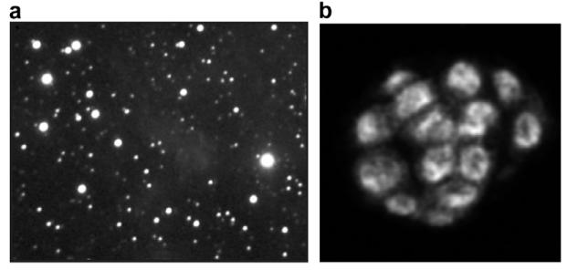
While the proposed technique focuses on biological data, its application is extensible to other data sets, such as stellar data, with blob-like signatures. With respect to biological data, subcellular regions have to be segmented for subsequent quantification of protein localization. Research in the segmentation of subcellular structures spans from traditional ad hoc methods of modeling intensity distribution to geometric techniques (Yang and Parvin, 2003; Parvin et al., 2007) and surface evolution methods (Chan and Vese, 2001; Raman et al., 2007). A key observation is that nuclear regions are often convex and form positive curvature maxima when they overlap each other. Our approach is based on constraining the solution to provide seeds corresponding to the nuclear regions and then breaking up local regions based on additional intensity and geometric constraints. The seeding is based on radial voting, where gradient information is projected inward to infer a local center of mass. Once these seeds are established, Voronoi tessellation provides the local neighborhood where each nucleus resides. This local neighborhood is further partitioned based on its intensity distribution using the level set methods. In summary, while voting methods offer robust model-based constraints for bounding the solution to the segmentation problem, level set methods offer numerically stable solutions to the active contour problems. By limiting and bounding the active contour model to a small nuclear region and its immediate background, a more stable solution is produced, which ensures that (1) overlapping compartments are not merged together, (2) potential leakage in the curve evolution is localized to a small neighborhood, and (3) an improved segmentation can be generated as a result of localized statistics of the region bounding one nucleus. The proposed technique is implemented and its performance is demonstrated on biological and stellar data as shown in Fig. 1.

Fig. 1.

Sample dataset: (a) stellar data with variable scale and intensity, and (b) a slice of a three-dimensional cell culture system with cells having variable size and intensity and overlapping compartments.

Organization of the paper is as follows: Section 2 provides a detailed description of the proposed method. Section 3 provides examples and results of the application of the proposed method on real data. Section 4 concludes the paper.

2. Approach

Specific steps in delineation of blob regions are shown in Fig. 2. With the 2D image as an input, the location of the centroid of each blob is estimated through iterative radial voting. With the estimation of these seeds, each blobs is bounded by Voronoi tessellation, which is further refined by active contour evolution.

Fig. 2.

Steps in delineation of blob regions in an image.

2.1. Review of segmentation with the active contour model

The active contour model has been used extensively in the imaging communities, and many variations of it are currently supported through ITK, from Kitware, Inc. The level set formulation (Osher and Sethian, 1988, 1992) of the active contour model offers a natural and numerically robust implementation of curve evolution equations within the Eulerian formulation. The ITK image library offers several 2D and 3D implementations of curve evolution within the level set framework. The most basic model includes a constant external motion coupled with geometric smoothing (Malladi et al., 1995). This model essentially behaves like a region-growing method, subject to the continuity of evolving contours while simultaneously handling topological changes. Another model within the ITK library, known as geodesic active contours (Caseless et al., 1997), aims to unify parametric and level set geometric models. This approach formulates the level set concept within an optimization framework. In addition, the ITK library includes a number of level set formulations of active contours that incorporate prior shape models, which can facilitate segmentation of known patterns. Our implementation corresponds to the Mumford-Shah function (Mumford and Shah, 1989) as modeled by Chan and Vese (2001) to segment objects whose boundaries are not necessarily defined by a gradient, thus reducing the leakage experienced by some gradient-based curve evolution functions. The deriving energy functions are governed by forces that are computed from the interior and exterior of evolving boundaries. A brief overview follows. The energy functional F(c₁, c₂, C) is defined by

$$\begin{array}{cc}\hfill F(c_1,c_2,C)=& \mu \cdot \text{Length}\left(C\right)+v\cdot \text{Area}\left(\text{inside}\left(C\right)\right)\hfill \\ \hfill & +{\lambda }_1{\int }_{\text{inside}\left(C\right)}{|u_0(x,y)-c_1|}^2\mathrm{d}x\mathrm{d}y\hfill \\ \hfill & +{\lambda }_2{\int }_{\text{outside}\left(C\right)}{|u_0(x,y)-c_2|}^2\mathrm{d}x\mathrm{d}y\hfill \end{array}$$ (1)

where u₀ corresponds to the image, c₁ and c₂ are the foreground and background intensity, and μ ≥ 0, v ≥ 0 λ, λ ≥ are fixed parameters. The level set formulation of this model is given by considering C ⊂ Ω as the zero-level set of a Lipschitz function ϕ : Ω → ℝ, in which Ω is a bounded open subset of ℝ². We refer the reader to Chan and Vese (2001) for more details. Using the Heaviside function H, and the one-dimensional Dirac measure δ₀, defined by

$$H\left(z\right)=\{\begin{array}{cc}1,\hfill & \text{if}z\ge 0,\hfill \\ 0,\hfill & \text{if}z<0,\hfill \end{array}\phantom{\}}{\delta }_0\left(z\right)=\frac{\mathrm{d}H\left(z\right)}{\mathrm{d}z}$$

The energy form can now be written as

$$\begin{array}{cc}\hfill F_{∊}(c_1,c_2,\varphi )=& \mu \int {\delta }_{∊}\left(\varphi (x,y)\right)|\nabla \varphi (x,y)|\mathrm{d}x\mathrm{d}y\hfill \\ \hfill & +v\int H_{∊}\left(\varphi (x,y)\right)\mathrm{d}x\mathrm{d}y\hfill \\ \hfill & +{\lambda }_1\int {|u_0(x,y)-c_1|}^2{H}_{∊}\varphi (x,y))\mathrm{d}x\mathrm{d}y\hfill \\ \hfill & +{\lambda }_2\int {|u_0(x,y)-c_2|}^2(1-H_{∊}\left(\varphi (x,y)\right))\mathrm{d}x\mathrm{d}y\hfill \end{array}$$ (2)

If ϕ is fixed then c₁ and c₂ can be expressed as

$$\begin{array}{cc}\hfill c_1\left(\varphi \right)& =\frac{{\int }_{\Omega }{u}_0(x,y)H_{∊}\left(\varphi (x,y)\right)\mathrm{d}x\mathrm{d}y}{{\int }_{\Omega }{H}_{∊}\left(\varphi (x,y)\right)\mathrm{d}x\mathrm{d}y}\hfill \\ \hfill c_2\left(\varphi \right)& =\frac{{\int }_{\Omega }{u}_0(x,y)(1-H_{∊}\left(\varphi (x,y)\right))\mathrm{d}x\mathrm{d}y}{{\int }_{\Omega }(1-H_{∊}\left(\varphi (x,y)\right))\mathrm{d}x\mathrm{d}y}\hfill \end{array}$$ (3)

and by keeping c₁ and c₂ fixed, the Euler-Lagrange equation for ϕ can be written as

$$\frac{\partial \varphi }{\partial t}={\delta }_{∊}\left[\mu \mathrm{div}\left(\frac{\nabla \varphi }{|\nabla \varphi |}\right)-v-{\lambda }_1{(u_0-c_1)}^2+{\lambda }_2{(u_0-c_2)}^2\right]$$ (4)

In our implementation, we have used the regularization of H, introduced by (Chan and Vese, 2001)

$$H_{∊}\left(z\right)=\frac{1}{2}\left(1+\frac{2}{\pi }\arctan \left(\frac{z}{∊}\right)\right)$$ (5)

While in some cases thresholding may be sufficient for colony segmentation, we have opted to use the active contour model since it is fast (about 1.8 s for an image of 512-by-512 with five colonies), avoids ad hoc parameter setting, and will be reused for nuclear segmentation. Examples are included in a later section.

2.2. Initialization with iterative scalar voting

Blob-like regions are convex and often radially symmetric, as shown in Fig. 1. Complexities arise as a result of non-uniform intensities, overlapping blobs, and variations in size. The underlying theme is to model the blob detection through perceptual grouping, thus making the detection more invariant to noise and variation in size. Voting along gradient direction provides a hypothesis profile for saliency, i.e. an approximate center of mass. While tensor voting (Medioni et al., 2000) provides grouping of co-directional features, it is non-iterative and may generate multiple seeds for blob detection. Furthermore, the notion of tensor voting is redundant because the voting is along the radial direction. In our implementation, the voting kernel is (i) scalar, (ii) designed in such a way that it encodes for a specific saliency, and (iii) refined iteratively. For example, the shape and evolution of these kernels for inferring center of mass is shown in Fig. 3, where voting is initiated along the gradient direction toward interior of the blob. Detection of radial symmetry is iterative, where gradient magnitude is projected along the radial direction according to a kernel function. The kernel function is smooth and its topography becomes more focused and dense at each iteration. Let I(x,y) be the original image, where the domain points (x,y) are 2D image coordinates. Let α(x,y) be the voting direction at each image point, where α(x,y): = (cos(θ(x,y)), sin(θ(x,y))) for some angle θ(x,y) that varies with the image location. Let {r_min, r_max} be the radial range and Δ be the angular range. Let V(x,y; r_min, r_max, Δ) be the vote image, dependent on the radial and angular ranges and having the same dimensions as the original image. Let A(x,y; r_min, r_max, Δ) be the local voting area, defined at each image point (x, y) and dependent on the radial and angular ranges, defined by

$$\begin{array}{cc}\hfill & A(x,y;r_{\min },r_{\max },\Delta )\hfill \\ \hfill & ≔\left\{(x\pm r\cos \varphi ,y\pm r\sin \varphi )\right|r_{\min }\le r\le r_{\max }\hfill \\ \hfill & \text{and}\theta (x,y)-\Delta \le \varphi \le \theta (x,y)+\Delta \}\hfill \end{array}$$ (6)

Finally, let K(x,y; σ, α, A) be a 2D Gaussian kernel with variance σ, masked by the local voting area A(x,y; r_min, r_max, Δ) and oriented in the voting direction α(x, y). Fig. 3 shows a subset of voting kernels that vary in topography, scale, and orientation (see Fig. 4).

Fig. 3.

Kernel topography: (a–e) Evolving kernel for the detection of radial symmetries (shown at a fixed orientation) has a trapezoidal active area with Gaussian distribution along both axes.

Fig. 4.

Evolution of radial voting on a nuclear image: (a) original image with edges being projected inward in the direction of the voting kernel; (b)–(d) voting landscapes from a subset of iterations. Notice that the initial bimodal voting landscape is eventually condensed into a single convex region.

The iterative voting algorithm is outlined below.

Iterative voting

• (1) Initialize the parameters: Initialize r_min, r_max, iΔ_max, and a sequence Δ_max = Δ_N > Δ_N−1 > … > Δ₀ = 0. Set n := N, where N is the number of iterations, and let Δ_n = Δ_max. Also fix a low gradient threshold, Γ_g and a kernel variance, σ, depending on the expected scale of salient features.

• (2) Initialize the saliency feature image: Define the feature image F(x,y) to be the local external force at each pixel of the original image. The external force is often set to the gradient magnitude or maximum curvature, depending upon the type of saliency grouping and the presence of local feature boundaries.

• (3) Initialize the voting direction and magnitude: Compute the image gradient, ∇I(x,y), and its magnitude, ǁ∇I(x, y)ǁ. Define a pixel subset S := {(x,y)|ǁ∇I(x, y)ǁ > Γ_g}. For each grid point (x,y) ∊ S, define the voting direction to be

  $$\alpha (x,y)≔-\frac{\nabla I(x,y)}{\parallel \nabla I(x,y)\parallel }$$
• (4) Compute the votes: Reset the vote image V(x,y; r_min, r_max, Δ_n) = 0 for all points (x,y). For each pixel (x,y) ∊ S, update the vote image as follows:

  $$\begin{array}{cc}\hfill & V(x,y;r_{\min },r_{\max },{\Delta }_n)=V(x,y;r_{\min },r_{\max },{\Delta }_n)\hfill \\ \hfill & +\underset{(u,v)\in A(x,y;r_{\min },r_{\max },{\Delta }_n)}{\Sigma }F\left(x-\frac{w}{2}+u,y-\frac{h}{2}+v\right)K(u,v;\sigma ,\alpha ,A),\hfill \end{array}$$

  where w = max(u) and h = max(v) are the maximum dimensions of the voting area.
• (5) Update the voting direction: For each grid point (x,y) ∊ S, revise the voting direction. Let

  $$(u^{\ast },v^{\ast })=\arg \underset{(u,v)\in A(x,y;r_{\min },r_{\max },{\Delta }_n)}{\max }V(u,v;r_{\min },r_{\max },{\Delta }_n)$$

  Let d_x = u^* − x, d_y = v^* − y, and

  $$\alpha (x,y)=\frac{(d_x,d_y)}{\sqrt{d_x^2+d_y^2}}$$

• (6) Refine the angular range: Let n:= n − 1, and repeat steps 4–6 until n =0.

• (7) Determine the points of saliency: Define the centers of mass or completed boundaries by thresholding the vote image:

  $$C=\left\{(x,y)\right|V(x,y;r_{\min },r_{\max },{\Delta }_0)>{\Gamma }_v\}$$

To illustrate the behavior of iterative voting, Fig. 5 shows intermediate steps that lead toward final results for overlapping 2D objects that are generated synthetically. The voting landscape corresponds to the spatial clustering that is initially diffuse and is subsequently refined and focused into distinct regions. Two examples of 2D voting are shown in Fig. 6, where each nucleus in a mammosphere has been detected.

Fig. 5.

Detection of radial symmetries for a synthetic image with multiple overlapping objects: (a) original image; and (b–d) voting landscape at several intermediate steps indicating convergence to a localized region.

Fig. 6.

Examples of voting applied to a stellar image (a) and slices of three-dimensional cell culture models.

2.3. Integrated voting and level set model

The voting results are used as vertices to generate a local neighborhood through Voronoi tessellation, as shown in Fig. 7. The Voronoi tessellation is a spatial decomposition of space, where the decomposition metric is defined to bisect distances to a specified set of objects. This local neighborhood is then used to constrain the blob segmentation within a small region. The actual segmentation is performed with the active contour model described earlier (Chan and Vese, 2001), and results are shown in Fig. 8.

Fig. 7.

Examples of Voronoi tessellation from voted blobs.

Fig. 8.

Examples of refined segmentation following Voronoi tessellation and level set.

3. Experimental results

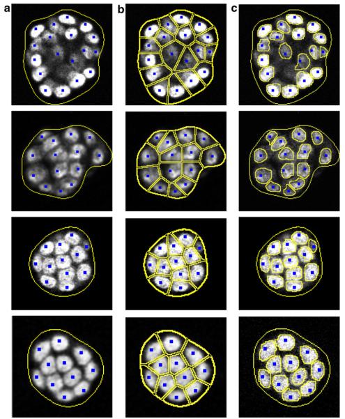
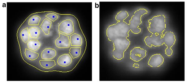
The proposed technique has been developed as a stand-alone package and being applied routinely for quantitative representation of three-dimensional cell culture (e.g., mammosphere) assays imaged with an epi-fluorescence microscope. A total of 74 images, corresponding to 152 colonies, were processed to evaluate the proposed segmentation approach. On average, each colony consisted of 16 cells, and the proposed segmentation algorithm had a 5% error in delineation due to excessive overlap between adjacent nuclei and non-uniform staining of nuclear regions. Fig. 9 shows several experimental results corresponding to noisy images, overlapping subcellular compartments, and variation in intensities. Nuclear detection through the voting method indicates high confidence, with only one cell to have been missed in the second image. This is due to the fact that only a small part of the cell is visible at this focal plane. The voting results serve as vertices to initiate Voronoi tessellation and a more detailed segmentation of the nuclear region. In Fig. 10, nuclear segmentation within the colony is shown without voting and tessellation for comparative analysis.

Fig. 9.

Several examples of low and high quality data: (a) The voting results; (b) corresponding Voronoi tessellation; and (c) final segmentation through level set method.

Fig. 10.

Comparison of segmentation in the absence of a local neighborhood established through Voronoi tessellation: (a) nuclear segmentation with the proposed method; and (b) segmentation results with only level set method applied within the colony.

4. Conclusion

We have shown that the traditional active contours are not appropriate for segmentation of heterogeneous blob features, where heterogeneity corresponds to variation in size and intensity of blobs that potentially overlap. But by constraining the active contour model to a local region, an improved solution can be realized. These local regions are estimated based on their aspect ratio having close proximity to unity; however, blobs can have internal structures, missing edges, and non-convex morphology. It is shown that scalar iterative voting provides an estimate for the center of mass, and that through Voronoi tessellation a local neighborhood can be constructed. Each local neighborhood constrains the active contour model to utilize the local image statistic and thereby improve segmentation. Application of this method to stellar and fluorescence cell based assay have been demonstrated.

References

- Caseless V, Kimmel R, Sapiro G. Geodesic active contours. Int. J. Comput. Vision. 1997;22(1):61–79. [Google Scholar]
- Chan T, Vese L. Active contours without edges. IEEE Trans. Image Process. 2001;10(2):266–277. doi: 10.1109/83.902291. [DOI] [PubMed] [Google Scholar]
- Malladi R, Sethian J, Vemuri B. Shape modeling with front propagation: a level set approach. IEEE Trans. Pattern Anal. Mach. Intell. 1995;17:158–175. [Google Scholar]
- Medioni G, Lee M, Tang C. A Computational Framework for Segmentation and Grouping. Elsevier; 2000. [Google Scholar]
- Mumford D, Shah J. Boundary detection by minimizing functional. Proc. Conf. Comput. Vision Pattern Recognition. 1985:22–25. [Google Scholar]
- Mumford D, Shah J. Optimal approximation by piecewise smooth functions and associated variational problems. Commun. Pure Appl. Math. 1989;42:577–685. [Google Scholar]
- Osher S, Sethian J. Front propagation with curvature dependent speed: Algorithms based on Hamilton–Jacobi formulation. J. Comput. Phys. 1988;79:12–49. [Google Scholar]
- Parvin B, Yang Q, Han J, Chang H, Rydbery B, Barcellos MH. Iterative voting for inference of structural saliency and characterization of subcellular events. IEEE Trans. Image Process. 2007;16:615–623. doi: 10.1109/tip.2007.891154. [DOI] [PubMed] [Google Scholar]
- Raman S, Maxwell C, Barcellos-Hoff M, Parvin B. Geometric approach segmentation and protein localization in cell culture assays. J. Microsc. 2007;225:22–30. doi: 10.1111/j.1365-2818.2007.01712.x. [DOI] [PubMed] [Google Scholar]
- Sethian J. Curvature and the evolution of fronts. Commun. Math. Phys. 1992;101:487–499. [Google Scholar]
- Shi J, Malik J. Normalized cut and image segmentation. IEEE Trans. Pattern Anal. Mach. Intell. 2000;22:888–906. [Google Scholar]
- Yang Q, Parvin B. Harmonic cut and regularized centroid transform for localization of subcellular structures. IEEE Trans. Biomed. Eng. 2003;50(4):469–476. doi: 10.1109/TBME.2003.809493. [DOI] [PubMed] [Google Scholar]
- Zhu S, Yuille A. Region competition: unifying snakes, region growing, and bayes/mdl for multiband image segmentation. IEEE Trans. Pattern Anal. Mach. Intell. 1996;18:884–900. [Google Scholar]