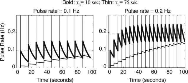
Figure 2.

Two examples of rate estimates in response to a regularly paced sequence of input pulses (here shown as finite-width rectangles). On the left, input pulses are widely spaced. The dashed line plots the actual rate of the pulses in pulses per second. On the right, a higher rate of pulses leads to a higher estimate, which oscillates around the true rate parameter (the dashed line). The results for two different time constants — τR = 10sec, bold; τR = 75sec, thin — are shown in both plots.
