

Abstract
Achieving atomic-level accuracy in comparative protein models is limited by our ability to refine the initial, homolog-derived model closer to the native state. Despite considerable effort, progress in developing a generalized refinement method has been limited. In contrast, methods have been described that can accurately reconstruct loop conformations in native protein structures. We hypothesize that loop refinement in homology models is much more difficult than loop reconstruction in crystal structures, in part, because side-chain, backbone, and other structural inaccuracies surrounding the loop create a challenging sampling problem; the loop cannot be refined without simultaneously refining adjacent portions. In this work, we single out one sampling issue in an artificial but useful test set and examine how loop refinement accuracy is affected by errors in surrounding side-chains. In 80 high-resolution crystal structures, we first perturbed 6–12 residue loops away from the crystal conformation, and placed all protein side chains in non-native but low energy conformations. Even these relatively small perturbations in the surroundings made the loop prediction problem much more challenging. Using a previously published loop prediction method, median backbone (N-Cα-CO) RMSD’s for groups of 6, 8, 10, and 12 residue loops are 0.3/0.6/0.4/0.6 Å, respectively, on native structures and increase to 1.1/2.2/1.5/2.3 Å on the perturbed cases. We then augmented our previous loop prediction method to simultaneously optimize the rotamer states of side chains surrounding the loop. Our results show that this augmented loop prediction method can recover the native state in many perturbed structures where the previous method failed; the median RMSD’s for the 6, 8, 10, and 12 residue perturbed loops improve to 0.4/0.8/1.1/1.2 Å. Finally, we highlight three comparative models from blind tests, in which our new method predicted loops closer to the native conformation than first modeled using the homolog template, a task generally understood to be difficult. Although many challenges remain in refining full comparative models to high accuracy, this work offers a methodical step toward that goal.
Keywords: comparative, homology, modeling, refinement, loop prediction, molecular mechanics, force field
INTRODUCTION
Despite the rapid increase in the rate of experimental protein structure determination catalyzed by structural genomics initiatives, the vast majority of known protein sequences will lack experimental structures for the foreseeable future. The ability to generate protein models comparable in accuracy to moderate-to-low resolution experimental structures for these proteins would have enormous utility for structure-based drug design and biological studies. Though the method of comparative (or homology) modeling is a useful tool in this regard, the resulting models vary in accuracy.1
Vitkup et al.2 estimated that 90% of all uncharacterized protein sequences within a protein family could be modeled, if on average two proteins per family are rationally selected for experimental structure determination. This suggests that, on average, about 100 protein sequences without any prior structural characterization could be modeled for each new experimental structure.1 The accuracy of these models, however, varies significantly. As documented by the New York Structural Genomix Research Consortium, many models accurately represent the overall tertiary structure, but relatively few (<10%, i.e., those with >50% sequence identity) are expected to be as accurate as moderate resolution experimental structures (1–2 Å RMSD).3 The majority of the models will require refinement in order to be useful for problems requiring high-resolution information, such as structure-based drug design.
There are two primary roadblocks to more reliably accurate comparative models, namely, difficulties in (1) identifying and aligning to a homolog template and (2) refining regions in the initial model that potentially differ structurally from the target protein. In general, while much progress has been made in the alignment step, little has been made in the refinement step.4–6 There are a number of approaches to refining protein models and we will not provide a detailed summary here. There has been some work to investigate the particular reasons for refinement difficulties. Fiser et al.7 predicted loops in structures with artificially distorted backbone positions in the environment of the loop and found that predictions became worse as expected. They suggested simultaneously optimizing the environment during the loop prediction to improve accuracy, but results were not shown. Qian et al.8 found that reducing the number of degrees of freedom, through sampling along principal components derived from protein family members, avoided generation of low energy, non-native models, and generally improved accuracy beyond the starting template. Mönnigmann and Floudas9 performed backbone sampling of residues flanking loops to account for flexibility and variation in the loop stems. Finally, Misura and Baker10 assessed the accuracy of their refinement methods on a test set of increasingly distorted starting structures by perturbing bond lengths, side chains and secondary structure elements, and finally on full de novo models. In general, they were able to refine the perturbed starting structures to lower RMSD models when compared to the native structure. They also found that most of the deviation in their models occurred in loop regions.
Two requirements for successful comparative model refinement are (1) efficient methods for sampling degrees of freedom that enable near-native configurations to be located from the starting structure; and (2) an energy function capable of identifying near-native conformations. Though some progress has been made,11–13 both of these challenges remain unsolved in our view. In this work, we take a simplified approach and focus exclusively on the sampling problem, in particular, through increased sampling within and around loop regions.
Most loop prediction algorithms have been evaluated primarily by their ability to reproduce the conformations of loops in protein crystal structures. In these tests, all portions of the protein other than the loop in question are generally retained in their native conformation, after adding hydrogen atoms and sometimes performing energy minimization. Numerous methods have been reported that achieve high-accuracy reproduction of loops in such tests.14–19,20 Accurate reconstruction of loops in crystal structures is an important prerequisite for the more challenging task of refining loops in homology models. The critical difference is that a given loop in a homology model will be surrounded by other portions of the protein that themselves are inaccurate. Refining the loop in this inaccurate environment, without explicitly optimizing the surroundings, frequently fails, indicating that loop refinement in homology models is much more difficult than loop prediction in crystal structures. The inaccuracies in the surroundings can be divided into three categories: (1) errors in the conformations of side chains surrounding the loop, (2) errors in the backbone flanking the loop (the loop “stems”), and (3) errors in nonadjacent portions of the backbone. In this work, we consider an artificial but useful intermediate case where we isolate only the first of these types of errors. That is, we have chosen to focus on loop prediction when side chains outside the loop have inaccurate initial conformations, but the backbone outside the loop is retained in the native conformation. This makes the loop prediction problem much more challenging, although still less difficult than loop refinement in homology models. We are not addressing larger refinement problems such as surrounding backbone, helix, or domain optimization. In doing so, we hope to de-convolute some of the causes of error and begin to bridge the gap between loop prediction in crystal structures and loop refinement in homology models.
We have developed a new method, Hierarchical Loop Prediction with Surrounding Side chain optimization (HLP-SS), for predicting loops in inexact environments that builds on a previously reported method, which we refer to here as Hierarchical Loop Prediction (HLP). Through the simultaneous optimization of side chains within and in the vicinity of the loop, we have increased the accuracy of our loop predictions relative to our previous protocol when applied to proteins with inaccurate surroundings. We previously applied a similar method to predicting loop conformational changes due to post-translational phosphorylation,18 an application with challenges that are similar to homology model refinement, but the approach has not otherwise been extensively tested. Here, we evaluate this protocol using a large and diverse test set of 80 loops, varying in length and difficulty, with artificially perturbed surroundings. We examine specific cases that illustrate successes and failures, and provide some anecdotal but encouraging results suggesting that the approach can be used successfully in blind tests of homology model refinement.
METHODS
In previous work,19 HLP, which is implemented in the Protein Local Optimization Program (PLOP), has been tested for its ability to reconstruct protein loops in crystal structures. The sampling algorithm and energy function have recently been improved20 for long loops as highlighted below. In this current work, we augment HLP by enabling the simultaneous sampling and optimization of surrounding side chains. A full description of the previous protocol can be found here.19,20 We provide an overview of HLP, and discuss the features of our new method, HLP-SS.
Previous hierarchical loop prediction method: HLP
The previously published method involves a hierarchy of loop prediction stages, in which the lowest energy loops generated from one stage are passed to the next where more focused (constrained) sampling is performed.
Specifically, as shown in Figure 1, the initial structure is passed to two, parallel, initial prediction stages (only one is shown) labeled “Init.” The two initial stages vary with the amount of allowed steric overlap between atoms as measured by an overlap factor: 0.7, 0.6, respectively. The overlap factor is defined as the ratio of the distance between two atom centers to the sum of their van der Waals radii. The resulting lowest five energy structures from each of the initial stages (10 total loops) are passed as new starting structures to the parallel refinement stages (only one is shown in Fig. 1). In the first refinement stage, the Cα atoms of the loop are constrained during sampling to less than 4 Å from Cα atoms in each starting loop. Finally, the five lowest energy loops from all refinement one stage processes are passed to five parallel refinement stages (only one is shown in Fig. 1) labeled “Ref. 2.” In this second refinement stage, the Cα atoms of the loop are constrained to less than 2 Å from Cα atoms in each starting loop. The lowest energy loop from all stages is taken as the predicted loop.
Figure 1.
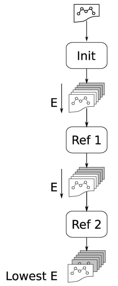
A high level schematic of the Hierarchical Loop Prediction (HLP) protocol described here and previously. “Init” refers to the initial stage of sampling and scoring. “Ref” refers to the refinement stages where sampling is constrained around starting loop conformations. See Methods for details.
An all-atom force field energy with implicit solvent is calculated for each sampled loop, and the loops are then ranked by energy. The energy is calculated using the Optimized Potential for Liquid Simulations (OPLS) all-atom force field,21–23 the Surface Generalized Born model of polar salvation,24 an estimator for the nonpolar component of the solvation free energy developed by Gallicchio et al.,25 and a number of correction terms as detailed in Ghosh et al.24 and in Jacobson et al.23
At each stage of the procedure, the sampling is performed by perturbing dihedral angles in the backbone and side chains, using knowledge-based preferences: as described previously,19 backbone dihedral angles are chosen randomly from a 5° resolution library representing the well-known Ramachandran plot, and side chain rotamers are chosen randomly from a 10° resolution library developed by Xiang and Honig.26 All heavy-atom torsion angles between the terminal peptide bonds are sampled. All bond lengths and angles associated with these are initially set to default values, but are allowed to vary during energy minimization. Polar hydrogens (e.g., OH group on Ser/Thr/Tyr) are sampled during side chain optimization; nonpolar hydrogens are not sampled other than through minimization.
To obtain greater accuracy for long loops (in this work, loops longer than nine residues), the algorithm has been augmented as described previously.20 Sampling has been increased dramatically through the addition of five additional “fixed” stages where subsegments of the loop are sampled, while the remainder of the loop is held fixed. In addition, Zhu et al. have also incorporated an additional hydrophobic term adapted from the Chem-Score27 scoring function, which has been successfully used to describe the hydrophobic contribution to the binding free energy between ligands and protein receptors. The “long loop” protocol and scoring function were utilized in this study for the 10 and 12 residue loop cases. We did not use the augmented protocol and energy function on the six and eight residue loop cases for efficiency reasons. Though, these changes have been applied to short loops in a previous study28 that shows moderate improvement in accuracy. Only three and four “fixed” stages were used for the 10 and 12 residue loop cases, respectively, to improve the computational efficiency. Our experience showed that this choice was sufficient to achieve convergent results.
New method incorporating surrounding side chains: HLP-SS
In this work, we modified the HLP algorithm presented above in two places: during the loop buildup and during the side chain optimization (Fig. 2).
Figure 2.
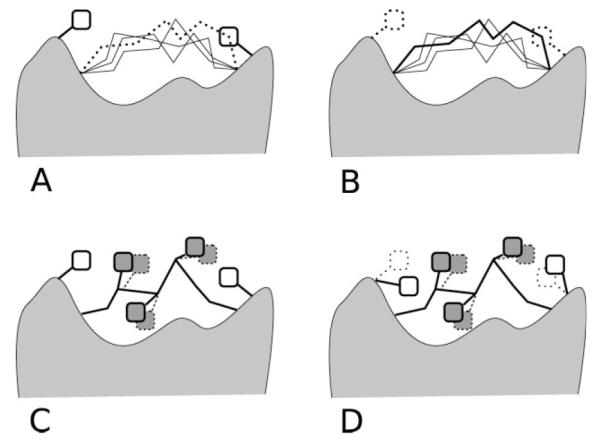
Schematic of the two ways surrounding side chains (white squares) are incorporated into each stage of our hierarchical protocol, backbone sampling (A and B) and simultaneous side chain optimization (C and D). (A) Our previous protocol HLP would eliminate loop backbones (dashed line) that overlap with surrounding side chain positions. (B) In an initial stage of HLP-SS, we remove the surrounding side chains (dashed squares) during backbone sampling to allow for backbone conformations that might be allowed if the surrounding side chains are given a chance to optimize. (C) HLP optimizes side chains on the loop only. (D) In HLP-SS, the side chains are optimized on the loop as well as the surrounding residues.
Removal of side chains during backbone sampling
For efficient backbone sampling, the previously published loop prediction method applies a variety of screens to rule out high energy loops as early as possible. One of these screens checks for steric clashes between the loop backbone and the rest of the protein, as the loop is built up from either side. By default, this steric screening checks for clashes with all heavy atoms outside the loop. However, if the portions of the model surrounding the loop are inaccurate, this screen could prevent native-like structures from being sampled, for example, if a side chain is occupying a portion of the space that the loop backbone should pass through. To avoid this problem, we created an option to ignore side chains surrounding the loop during the steric screening.
However, a significant downside to ignoring the surrounding side chains during backbone sampling is that the conformational search space increases significantly. Also, we may be discarding information because frequently, some initial side chain conformations in the surroundings are approximately correct. For any given loop refinement in a particular model, it is not a priori obvious whether including or excluding surrounding side chains is more likely to succeed. For this reason, in our method, we do both (in separate optimizations) and ultimately use the MM-GBSA energy function implemented in PLOP to choose the final predicted conformation. Specifically, we added a third initial stage “Init3” with overlap factor of 0.7, and used our new option to exclude surrounding side chains during the steric screening. We continue to include the surrounding side chains during steric screening in the original two initial stages, “Init1” and “Init2.” Finally, we also make certain to optimize the same surrounding side chains across all prediction stages, so that we can compare the energies of all sampled loops.
Simultaneous optimization of side chains in surroundings and loop
In the HLP method, the energy for each candidate loop conformation is obtained after iteratively optimizing the side chain conformations on the loop followed by energy minimization. In the HLP-SS, we expand the list of side chains to be optimized by including the side chains of the surrounding residues. The self-consistent side chain optimization is accomplished by iteratively placing one side chain at a time, while holding the others fixed until no side chain changes rotamer state. In HLP-SS, we optimize the side chains on the loop first and then side chains from surroundings, iteratively.
Data set choice and perturbation
To de-convolute the many compounding problems that occur in loop prediction in full comparative models, we chose to predict loops on a data set consisting of crystal structures that are perturbed to contain modeling errors in side chains only. Our current goal is neither to create a representative sampling of all loops found within proteins nor to generate all possible loop refinement scenarios found in comparative models. Rather, our intention is to create a test set with enough variety in difficulty and types of refinement problems, that we (and others) may test approaches to loop prediction in inaccurate environments.
Criteria for test set selection
We constructed a test set of 80 loops, 20 loops each of 6, 8, 10, and 12 residues in length. For each loop length, we chose a smaller number of loops from the larger, previously published sets19,20 due to the computational expense of the additional sampling of the loop surroundings. The 6, 8, and 10 residue loops were taken from Jacobson et al.19 and the 12 residue loops were taken from Zhu et al.20 The proteins in the set are diverse in sequence, observed in crystal structures with <2.0 Å resolution, and have been filtered such that the simulated loops are far from heteroatom groups. This set contains a mix of both difficult and easy loop prediction cases, similar to the previously published larger test sets. The median RMSD predictions for our subset of loops are similar to those from the larger, previously published test sets (when predicted on the native crystal structure with simulated crystal environment).
Generation of perturbed crystal structures
We perturbed crystal structures in the following way. For each of the 80 loops, we performed the following.
Generate a low-energy loop far from the native conformation
We performed a single run of loop prediction in PLOP that generates a list of sampled loops ranked by MM-GBSA energy. In general, we chose a sampled loop greater than 3 Å backbone heavy atom RMSD from the native loop and then grafted this loop onto the crystal structure. In some cases, no loops were sampled greater than 3 Å from the native and in those cases, we simply selected from one of the lower-RMSD, non-native loops.
Rotamer optimization on the full protein with non-native loop
We performed rotamer optimization and energy minimization on all side chains in the perturbed protein using the method described in Jacobson et al.19 This procedure removes the memory of native χ angles and bond lengths/angles of all side chains and places the protein in a non-native, local minimum, creating a more difficult loop prediction scenario that more closely resembles an initial comparative model.
The dataset and the relevant information are listed in Tables S1, S2, S3, and S4.
Method of choosing surrounding side chains to optimize
The key new element introduced into the loop modeling procedure is simultaneous optimization of side chains on the loop and in its surroundings. In the extreme, the algorithm could optimize all side chains on the protein, but this would unnecessarily increase computational expense due to sampling many side chains distant from the loop (and also increases “noise” in the computed energy). At the other extreme, only those side chains in contact with the starting loop could be optimized. However, the initial loop may be far from its native position in a homology model, as are many of the perturbed loops in our test set. For this reason, we developed a protocol to attempt to identify all side chains that could interact with any conformation of the loop. We accomplish this by first generating a coarse unbiased sampling of loops, <50, using a quick backbone buildup within PLOP. We then identify all residues with a distance cutoff of any of these loop conformations to decide which side chains outside the loop are optimized. Surrounding residues are included that have a side-chain heavy atom within a certain cutoff from Cβ atoms within an initial set of sampled loops. The Cβ atoms from the N-terminal and C-terminal loop residues are excluded in this screen. For example, at a distant cutoff of 7.5 Å, this translates to an average of 17 surrounding side chains for the 8-residue cases, but the number varies considerably from 9 to 37 depending on the solvent-exposure of each loop. We tested distance cutoffs of 5.0, 7.5, and 10.0 Å in this work.
Sampling and energy function failure analysis
In cases where the method predicted loops greater than 1.5 Å backbone heavy atom RMSD, we attempted to understand why, distinguishing between two broad classes of problems: insufficient sampling and inability of the energy function to identify near-native states. Sampling problems were identified if no loops are sampled within 1 Å N-Cα-C RMSD from the native. Energy function problems are identified by calculating Egap, the difference in energy between our predicted loop and a native-like loop. We did not calculate the native energy using the conformation found in the crystal structure because the loop found in the crystal structure must relax using the same optimizations as our predicted loops in order for the energies to be comparable. The native energy is taken from the lowest energy loop with <1 Å N-Cα-C RMSD from the native. For consistency, this analysis was carried out on both the unperturbed and perturbed crystal structure test cases.
RMSD calculations
Loop RMSD’s are calculated using N, Cα, C, and O atoms in the loop backbone with the protein aligned, excluding the loop. Side chain RMSD’s are calculated using non-hydrogen atoms in the side chain. Full comparative models were first aligned to the native crystal structures using the MatchMaker function in Chimera29 with default settings.
Crystal packing simulation
We do not include crystal packing in the primary predictions presented here. However, in one case we suspected crystal packing effects might affect the results, and to investigate this possibility, we used the option in PLOP that includes all atoms found in a single asymmetric unit plus all atoms <20 Å from adjacent asymmetric units. Each asymmetric unit is identical at every stage of the calculation.
Protonation states of titratable residues
All titratable residues are placed in their standard protonation state at pH 7.0 (e.g., histidine is neutral), regardless of whether pH is specified in the PDB file. This assumption may affect accuracy in some cases, particularly, when we compare to structures that were crystallized at nonphysiological pH.
Generation of full comparative model test set
To begin to test the applicability of our new method in full comparative models, we refined loops within initial models that were generated by our team in the latest Critical Assessment of Techniques for Protein Structure Prediction (CASP7) experiment.30 As the submitted models highlighted here were refined using HLP-SS, the refinements were “blind” tests. Targets T326, T345, and T376 are highlighted in this work. Target T326 was aligned to template, 2GHR, using BLAST31 and constructed using PLOP19 as previously described.32 T345 and T376 were aligned to templates 2F8A and 1YXC, respectively, using HMAP33 and constructed using NEST.33 A loop was identified in the initial model as “requiring refinement,” if the sequence alignment between template and target contained gaps or deletions within regions between secondary structure elements found in the template structure.
RESULTS AND DISCUSSION
Assessment of our previous method: HLP
A comparison of results applying our previous protocol, HLP, to the unperturbed and perturbed test cases illustrates how incorrect side chain conformations can degrade the performance of loop predictions when surrounding side chains are not included in the optimization (Table I). For all loop lengths, the median backbone RMSD increases by approximately a factor of 4. More specifically, HLP predicts 42 out of 80 test cases greater than 1.5 Å backbone RMSD on the perturbed test set compared to 15 out of 80 when predicted on the unperturbed crystal structures. The “easy” test cases, that is, the ones that the previous protocol performs relatively well on, serve as controls to verify that our new protocol does not adversely affect these cases.
Table I.
Median and Average Predicted Loop Backbone (N-Cα-C-O) RMSD’s in Å Using our Previous and New Methods on Unperturbed and Perturbed Crystal Structure Test Cases
| Crystal structures |
Perturbed crystal structures |
||||||||
|---|---|---|---|---|---|---|---|---|---|
| 6 res. | 8 res. | 10 res. | 12 res. | 6 res. | 8 res. | 10 res. | 12 res. | ||
| Starting structures | Median RMSD | 0.0 | 0.0 | 0.0 | 0.0 | 2.9 | 3.9 | 4.2 | 4.8 |
| Average RMSD | 0.0 | 0.0 | 0.0 | 0.0 | 3.4 | 4.3 | 4.9 | 4.6 | |
| HLP | Median RMSD | 0.3 | 0.6 | 0.4 | 0.6 | 1.1 | 2.2 | 1.5 | 2.3 |
| Average RMSD | 0.7 | 1.2 | 0.6 | 1.2 | 1.7 | 2.4 | 1.7 | 2.6 | |
| Sampling failures | 1 | 3 | 0 | 0 | 3 | 9 | 6 | 6 | |
| Energy failures | 1 | 2 | 1 | 7 | 4 | 4 | 4 | 6 | |
| HLP-SS | Median RMSD | 0.4 | 1.0 | 0.8 | 0.9 | 0.4 | 0.8 | 1.1 | 1.2 |
| Average RMSD | 0.8 | 1.4 | 1.0 | 1.4 | 0.8 | 1.3 | 1.5 | 1.7 | |
| Sampling failures | 0 | 0 | 0 | 4 | 0 | 1 | 0 | 2 | |
| Energy failures | 3 | 6 | 4 | 3 | 3 | 3 | 7 | 6 | |
Statistics are calculated over the 20 test cases in each loop-length category. The numbers of sampling and energy failures are also listed. Rows 1 and 2, the median and average RMSD of the loop before prediction. Rows 3 and 4, median and average RMSD for predictions using HLP (without optimizing surrounding side chains). Rows 5 and 6, the number of sampling and energy failures in each subset using HLP. Rows 7 and 8, median and average RMSD for predictions using HLP-SS (optimizing surrounding side chains). Rows 9 and 10, the number of sampling and energy failures in each subset.
Using HLP on perturbed structures, we anticipated a decrease in accuracy due to sampling since the perturbed side chains in the surroundings of the loop may block the native conformation. Interestingly, the number of energy function problems also increases, indicating that native-like loop backbones are being sampled using our old protocol, but the perturbed surroundings may be preventing key side chain contacts from forming.
Assessment of our new method: HLP-SS
To test whether our new protocol, HLP-SS, is more effective at predicting loops in inexact environments, we utilized our perturbed test set and compared results using HLP-SS to results using HLP.
We first varied the number of surrounding side chains to include during the loop prediction by testing our new protocol with different cutoff distances (see Methods). The comparison of prediction accuracy to computational expense summarized in Figure 3 indicates that a radius of 7.5 Å is a good tradeoff. Interestingly, increasing the radius to 10 Å does not give a marked increase in accuracy over a radius of 7.5 Å but does increase computational expense considerably. All results in this article are reported using the 7.5 Å cutoff, unless otherwise noted.
Figure 3.
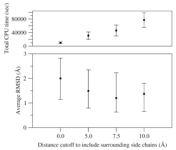
Comparison of total relative CPU time (top) and prediction accuracy (bottom) versus increasing cutoff distance for including surrounding side chains using HLP-SS. The radii cutoffs of 0.0 (i.e., none), 5.0, 7.5, and 10.0 Å specify that surrounding residues are included in the optimization (see Methods). Top: Average total CPU times in seconds represent a relative cumulative time if our new protocol were not run in parallel. For clarity, average CPU times are shown for the 20 eight-residue test cases only. Error bars represent the standard deviation across each data set. Bottom: Average RMSD’s are calculated over all test cases. Positive and negative error bars contain 34.1% of the RMSD population above and 34.1% below the average, respectively.
The results in Table I show a consistent increase in accuracy when side chains surrounding the loop are optimized during the loop prediction compared to when they are held fixed. Individual predictions can be found in the supplemental Tables S1, S2, S3, and S4. The overall accuracy for each loop length is increased using HLP-SS over HLP. For example, for the eight residue perturbed loop set, the median backbone RMSD is 0.8 Å using HLP-SS compared to 2.2 Å using HLP. By comparison, on the unperturbed eight residue loops, the median backbone RMSD is 1.0 Å using HLP-SS and 0.6 Å using HLP. Thus, the results of using HLP-SS on the perturbed loops approaches the accuracy that can be achieved in loop reconstruction, especially for short loops (six and eight residues). With longer loops (10 and 12 residues), HLP-SS produces a small increase in median backbone RMSD (by a factor of ~1.3) on perturbed structures versus unperturbed. Including surrounding side chains during the loop optimization clearly produces more accurate results on our perturbed test set than not including them.
The number of sampling problems is reduced using our new method: out of the 80 perturbed test cases, HLP produces 24 loop sampling problems compared to three using HLP-SS (see Methods for our definition of sampling and energy problems). HLP-SS produces similar numbers of sampling problems as seen in the control experiments on the unperturbed crystal structures. These results suggest (1) our perturbed test set creates more sampling difficulties than the unperturbed crystal structures, and (2) our enhanced sampling in the HLP-SS method is addressing these difficulties. However, the number of errors that can be attributed to limitations of the energy function is not reduced using HLP-SS. In loop reconstruction in native crystal structures, the number of failures attributed to the energy function increases using HLP-SS versus HLP. That is, the increased sampling due to simultaneous optimization of side chains surrounding the loop places a greater burden on the energy function in distinguishing between native and non-native configurations (i.e., many more non-native side chain contacts are sampled). Thus, the perturbed loop test set increases the difficulty of both sampling native-like configurations and identifying these among many non-native conformations, relative to loop reconstruction in native proteins.
As a control, we tested our new method on native crystal structures to see if our new method degrades accuracy when the loop and its surroundings are initially in the native state. This control represents the “best that we can expect” using HLP-SS because it will uncover energy and sampling problems unrelated to the altered side chains in the perturbed test set. As expected, median backbone RMSD’s increase slightly using HLP-SS compared to HLP: results using HLP-SS show an increase of +0.1, +0.4, +0.4, and +0.3 Å for 6, 8, 10, and 12 residue loops respectively over HLP (Table I). Sampling surrounding side chain rotamers increases the number of degrees of freedom and thus the likelihood of energy function or sampling problems.
If we consider the set of “easy loops” among the perturbed loop test set, that is, cases where our old protocol predicts native-like loops (better than 1.5 Å backbone RMSD), our new protocol predicts non-native loops (worse than 1.5 Å RMSD) in only 5 of these 39 easy cases.
Interestingly, although the average loop prediction accuracy improves with our new method, the average accuracy of the side chains in the surroundings does not improve (data not shown). Looking at averages over many surrounding residues may be hiding the role of an important few. Although in some cases the role of a single surrounding residue is clear, such as in case 1CLC (see below) where a single residue blocks sampling of the native conformation, other cases are more subtle. In cases where sampling is not a problem, key energetic contributing residues, now free to move in our new method, may form incorrect contacts for reasons such as differences in the pH between crystal structure and our modeling conditions, or other problems with our energy function.
Effects of crystal packing
Because our goal is to predict loops within comparative models, where crystal symmetry information is not known, we do not simulate the crystal environment in the primary predictions presented here. However, since we are comparing to crystal structures in this intermediate step, crystal packing effects may contribute to apparent error in our predictions.19,34 To assess these effects in our test set, we performed predictions using HLP on the unperturbed crystal structures with and without simulation of crystal packing (Table S5). Simulation of crystal packing is described in Methods. Nine cases (PDB’s: 1XIF, 3TGL, 1IAB, 1PRN, 1SBP, 1ARB-12 residue case, 1CNV, 1M3S, 1OTH) show potential crystal packing effects that we define as a predicted loop backbone accuracy >1.5 Å RMSD without simulating crystal packing but <1.5 Å RMSD with crystal packing. Loop predictions are affected by either restricting the sampling space or by changing the energy landscape through inter-chain contacts. Since HLP is sampling conformations <1.2 Å RMSD in all nine cases without simulated crystal packing, the increases in accuracy with crystal packing are probably not due to restricting the sampling space but are enabled through inter-chain energetic contacts. See example 3TGL below for an example.
Most importantly, these errors likely propagate through our perturbed test predictions and should be taken into account in assessing the new method. However, removing the above nine cases (identified as having adverse crystal packing effects) from our statistics, we see little increase in overall accuracy for our new method (Table S6). HLP-SS median RMSD’s for the 6, 8, and 10 residue perturbed cases stay within 0.1 Å of the statistics derived from the full test set, suggesting crystal packing is playing a minor role for the cases. Because four of the nine “crystal packing” cases are in the 12 residue test set, the statistics show moderate decreases in median and average RMSD’s for both our old and new protocol. In the 12 residue perturbed test set, median/average RMSD’s for HLP-SS are reduced from 1.2/1.7 to 1.1/1.3 Å in this filtered test set. Statistics for HLP are reduced from 2.3/2.6 to 1.6/2.4 Å.
1CLC
The benefits of our approach are clear in the eight residue test case 1CLC, residues 313–320. In the perturbed loop starting structure, Glu322 protrudes into the space that the native loop would occupy (Fig. 4). Without optimizing this side chain during the loop prediction, near-native loops will have high energies due to steric clashes. HLP-SS selects a near native loop with backbone RMSD of 0.4 Å. Without side chain optimization, the lowest energy loop is 4.3 Å RMSD. Sampling is enhanced near the native as seen in Figure 5.
Figure 4.
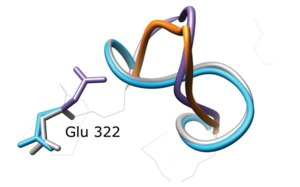
A successful application of our algorithm in PDB 1CLC, residues 313–320. The crystal structure is in gray, the initial perturbed structure is in purple, the predicted loop using our old protocol is in orange and our prediction using surrounding side chain optimization during loop prediction is in light blue. Glu322 partially obstructs the native loop conformation in the initial perturbed starting structure. A near-native loop is only correctly predicted when nearby side chains including Glu322 are also optimized.
Figure 5.

Calculated MM-GBSA energy versus loop N-Cα-C RMSD between predicted and native loop conformations for test case 1CLC. Only samples within 50 kcal/mol of the lowest predicted energy are shown. Top: predicting loops without nearby side chain optimization (HLP method). Bottom: predicting loops with nearby side chain optimization (HLP-SS method). Note since different atoms are optimized in each example, the relative shapes, and not absolute energies, between the two plots are comparable.
1F46
Another successful prediction, the 12 residue test case 1F46 (residues, 64–75), highlights a more subtle effect of incorrect surroundings on loop refinement. HLP-SS predicts a 1.1 Å backbone RMSD loop, while HLP predicts a 3.8 Å backbone RMSD loop (Fig. 6). In contrast to 1CLC above, there are no surrounding side chains obstructing the backbone from sampling close to the native. As seen using HLP, backbone conformations are sampled as low as 0.3 Å RMSD. HLP selects a 3.8 Å RMSD loop because at least one incorrect surrounding residue prevents a key loop side chain from repacking, thus leading to near-native conformations having high energies. Interestingly, HLP-SS with a 5.0 Å cutoff also failed, predicting a loop of 2.3 Å RMSD. By examining which residues are included in the 7.5 and 5.0 Å cutoffs, we determined that the repacking of the side chain of Met64 is blocked by nearby Arg161, a residue that is not optimized in the HLP and HLP-SS (5.0 Å cutoff) protocols. Optimizing Arg161 with the larger 7.5 Å cutoff enables repacking of Met64 and contributes to a lower energy, near-native loop.
Figure 6.
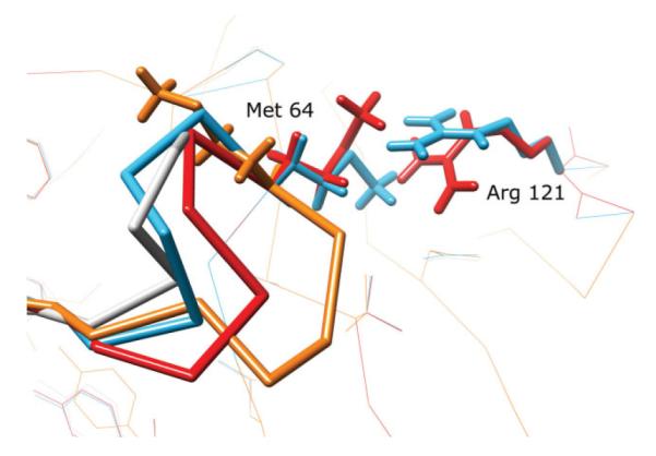
Comparison of loop predictions on the 12 residue loop test case, PDB 1F46, residues A:64-A:75. The crystal structure is in gray, the predicted loop using our old protocol, HLP, is in orange, our prediction using HLP-SS using a side chain cutoff of 5Å is in red and our prediction using HLP-SS with a side chain cutoff of 7.5 Å is in light blue. Heavy atom backbone RMSD’s are HLP: 3.8 Å, HLP-SS (5.0 Å cutoff): 2.3 Å, HLP-SS (7.5Å cutoff): 1.1 Å. The Arg121 residue outside the loop is not optimized in either the HLP or HLP-SS (5.0 Å) protocols.
3TGL
Including surrounding side chains did not improve our prediction of the six residue loop, residues 82–87 in 3TGL, beyond 3.1 Å backbone RMSD. Upon inspection of the original crystal structure, we found significant interactions between the loop and other chains within the asymmetric unit. We thus reran our calculations, while including all atoms from crystal symmetry chains within 20 Å of the original chain. Note that the 7.5 Å cutoffs for including nearby side chains was reapplied to capture residues from the symmetry copies of the protein. Our new prediction achieved a 0.5 Å backbone RMSD and correctly forms the salt bridge between Arg86 and Glu47 of the symmetric chain (Fig. 7). In a control experiment using HLP on the unperturbed crystal structure, the effect of crystal packing is clear with accuracy increasing from 3.1 to 0.7 Å when crystal packing is simulated. The apparent failure of HLP-SS to predict the native loop in the perturbed 3TGL structure is therefore due to crystal packing.
Figure 7.

The loop in 3TGL, residues 82–87, is shown with our predictions in light blue and crystal structure in gray. Top: our new protocol predicts a conformation with a backbone RMSD of 3.1 Å. Bottom: by including the additional atoms from the surrounding chains in the crystal, our new protocol predicts a near-native loop with 0.7 Å backbone RMSD.
1ALC
HLP-SS failed to identify a native loop in the eight residue loop case, PDB 1ALC. This target was identified as problematic even when predicting the loop within the native crystal structure but the failure is not due to omission of crystal packing. Although we sampled a loop as close as 0.4 Å backbone RMSD (Fig. 8, black triangles), we were not able to identify it as a near native loop because its energy is higher than decoy loops with >4.0 Å backbone RMSD from the native. In this case, the failure does not appear to be due to limitations of the energy function but rather due to a particularly rugged energy landscape for this loop. Though the loop is on the protein surface, a large percentage of its surface area is buried (Fig. 9). To validate this idea, we reran our prediction while constraining the sampling within 1 Å of the native loop and successfully identified a near-native loop lower in energy than the previously generated decoys (Fig. 8, red circles). In the future, optimizing the surrounding backbone atoms in addition to side chains may improve sampling for loops like this that are tightly constrained by their environment.
Figure 8.
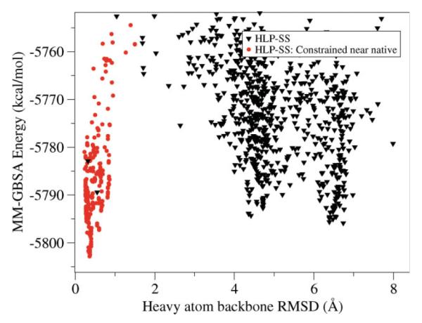
In black triangles, the MM-GBSA energy is plotted versus N-Cα-C RMSD for each sampled loop conformation using our HLP-SS applied to loop residues 34–41 in PDB 1ALC. Though one loop conformation with loop backbone RMSD of 0.3 Å is sampled, lower energy decoys exist with backbone RMSD greater than 4.0 Å from the native. In red, energy versus backbone RMSD for sampled loops constrained to less than 2.0 Å from the native.
Figure 9.
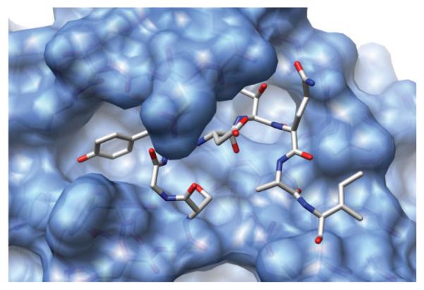
Depiction of the crystal structure, PDB 1ALC. The native loop, residues 34–41, sits in a tight pocket. All atoms not in the loop are represented as a blue surface map, while the loop surface has been removed to show the environment in which we are sampling.
Application of our new method to the refinement of full comparative models
To begin testing whether our new method can better refine full comparative models, where backbone as well as side chain atoms are inexact, we compared results from loop predictions on three homology models using our old and new methods. The resulting models using HLP-SS were submitted to the CASP7 experiment. After the experiment, we reran the loop refinements using HLP to compare to our blind HLP-SS results.
The important question is whether each method predicted loops more accurate than the initial homolog-derived loop, a task generally considered to be difficult. Figure 10 and Table II clearly show that ignoring surrounding side chains produced less accurate predictions than the initial starting models: HLP results for targets T345, T326, and T376 were 5.6, 2.2, and 5.6 Å RMSD respectively in comparison to the starting conformations, 1.5, 1.7, and 4.6 Å RMSD. In contrast, HLP-SS not only produced more accurate loops than HLP, it also improved somewhat upon the starting loop in these cases: HLP-SS predicts loops to 1.4, 1.1, and 3.5 Å backbone RMSD for the three targets.
Figure 10.

Comparison of blind loop predictions within full comparative models to native crystal conformations. In all figures, the loops are colored as follows. Gray: native crystal structure, Purple: unrefined loop model, Orange: refined loop model without simultaneous optimization of surrounding side chains, Blue: refined loop model with simultaneous optimization of surrounding side chains. Top: CASP7 target T345, residues 11–19. Middle: CASP7 target T376, residues 273–284. Bottom: CASP7 target T326, residues 173–178.
Table II.
Loop Predictions on Full Comparative Models
| Model | Native PDB |
Loop start residue number |
Loop end residue number |
Starting loop RMSD |
Predicted loop RMSD: HLP |
Predicted loop RMSD: HLP-SS |
|---|---|---|---|---|---|---|
| T345 | 2HE3 | 11 | 19 | 1.5 | 5.6 | 1.4 |
| T326 | 2H2W | 173 | 178 | 1.7 | 2.2 | 1.1 |
| T376 | 2HMC | 273 | 284 | 4.6 | 5.6 | 3.5 |
Column 1, CASP model designation; Column 2, the native PDB; Columns 3 and 4, the loop endpoints; Column 5, the starting backbone heavy atom (N-Cα-C-O) RMSD; Column 6, the predicted backbone RMSD using our old protocol that does not optimize surrounding side chains; Column 7, the predicted backbone RMSD using our new protocol that simultaneously optimized the surrounding side chains. Each model was first globally aligned to the crystal structure using Chimera to calculate RMSD’s.
Our intention here is to highlight evidence that initial models with both backbone and side chain errors can also benefit from HLP-SS. We do not make the claim that our protocol will work on all comparative models and we have seen many cases, where backbone perturbations outside of the loop are large enough that HLP-SS fails (data not shown). However, the difficulty of homology model refinement is such that any success in a blind test is encouraging. At the very least, these examples highlight how loop prediction methods that do not account for errors in the surroundings (HLP in this work) not only fail to improve homology models but can make the results much worse.
CONCLUSION/FURTHER DIRECTIONS
Refining comparative models is difficult for two reasons: the energy landscape is rugged and the sampling space is vast. In this study, we aimed to address one important sampling difficulty that occurs in the refinement of protein models, namely the ab initio prediction of loop segments when surrounding residue side chain positions are incorrect. By sampling rotamer states of nearby residues simultaneously with our previous all-atom loop sampling strategy, we have shown that a simple solution can significantly improve our predictive ability in these cases.
We chose to test our protocol on perturbed crystal structures. Rationally perturbed, idealized test sets are critical to de-convolute the sources of difficulty facing full comparative modeling refinement. In this study, we show that simply perturbing loops and then scrambling side chains in crystal structures creates a much more difficult loop prediction problem, relative to reconstructing loops in unperturbed crystal structures. We then show that our new method can predict near-native loops in a large majority of these perturbed cases by simultaneously sampling the side chains surrounding the loop. Our 80 perturbed test cases are available for download (see link below).
A logical next step after perturbing side chains within crystal structures is to introduce inaccurate backbone conformations in regions of the protein surrounding the loop in question. Initial results (data not shown) suggest that optimizing backbone atoms in surrounding residues, including the loop “stem” residues, during the side chain optimization stage can improve predictions in cases where surrounding inaccuracies cannot be corrected through side chain optimization alone.
Increasing the sampled degrees of freedom as we have done in this study implies a need for an energy function that is increasingly more robust at discerning native-like from non-native-like structures. Robust homology model refinement will thus require not only the development of new sampling methods but also more accurate energy functions. Some limitations are addressable whereas others are not. For example, because we are comparing our predictions to experiments, experimental factors that are not generally known at the time of comparative modeling can affect our accuracy. We have shown (Fig. 7 and Table S5) that inclusion of the crystal symmetry chains during the loop prediction can increase accuracy. The pH at which the protein was crystallized can also dramatically affect conformations seen in the crystal structure, particularly with side chain positions relevant to this current study. Since we assumed standard protonation states for titratable residues at pH 7.0, we will not account for changes in conformation due to pH.
There are energy function limitations we can improve without knowledge of experimental crystal conditions, however. Though we can only assume a physiological pH at the time of modeling, we should be able to predict local pKa shifts within the protein. We hope to address this issue in the near future. Limitations in using the Generalized Born implicit solvent model can lead to over-stabilized salt bridges35 and will fail to predict water-mediated interactions. Using a fixed-charge, non-polarizable force field may introduce errors as well.
An assumption implicit in this work is that the loop adopts a single well-defined conformation, and that the correct answer is the single conformation reported in the PDB file. From a computational standpoint, this limitation can be addressed by recasting the algorithms presented in this work as Monte Carlo sampling, that is, to predict an ensemble of structures rather than a single structure. Work along these lines is underway. Predicted ensembles of loop structures could be compared to experimental temperature factors from crystal structures, or preferably, to structures that were refined using an ensemble approach.36
Supplementary Material
ACKNOWLEDGMENTS
The authors thank David Pincus for early work and discussion which guided much of this work. They also thank Andy Kuziemko from the Barry Honig lab for providing the initial comparative model T376 for the “applications” section of this study. Finally, they thank the entire Barry Honig and Richard Friesner labs for their support during CASP7. MPJ is a member of the Scientific Advisory Board of Schrodinger Inc. Molecular graphics images were produced using the UCSF Chimera package from the Resource for Biocomputing, Visualization, and Informatics at the University of California, San Francisco. Our test set of perturbed crystal structures can be downloaded here: http://jacobson.compbio.ucsf.edu
Grant sponsor: NIH; Grant numbers: GM52018, GM81710, P41 RR-01081; Grant sponsors: Sandler Program in the Basic Sciences, Sloan Foundation, Genentech Scholars Program; Grant sponsor: NSF; Grant number: MCB-0346399.
Footnotes
The Supplementary Material referred to in this article can be found online at http://www.interscience.wiley.com/jpages/0887-3585/suppmat/
REFERENCES
- 1.Baker D, Sali A. protein structure prediction and structural genomics. Science. 2001;294:93–96. doi: 10.1126/science.1065659. [DOI] [PubMed] [Google Scholar]
- 2.Vitkup D, Melamud E, Moult J, Sander C. Completeness in structural genomics. Nat Struct Biol. 2001;8:559–566. doi: 10.1038/88640. [DOI] [PubMed] [Google Scholar]
- 3. Available at http://www.nysgrc.org/.
- 4.Moult J. A decade of CASP: progress, bottlenecks and prognosis in protein structure prediction. Curr Opin Struct Biol. 2005;15:285–289. doi: 10.1016/j.sbi.2005.05.011. [DOI] [PubMed] [Google Scholar]
- 5.Moult J, Fidelis K, Rost B, Hubbard T, Tramontano A. CASP introduction: critical assessment of methods of protein structure prediction (CASP)—round 6. Proteins. 2005;61:3–7. doi: 10.1002/prot.20716. [DOI] [PubMed] [Google Scholar]
- 6.Tress M, Ezkurdia I, Graña O, López G, Valencia A. Assessment of predictions submitted for the CASP6 comparative modeling category. Proteins. 2005;61:27–45. doi: 10.1002/prot.20720. [DOI] [PubMed] [Google Scholar]
- 7.Fiser A, Do RK, Sali A. Modeling of loops in protein structures. Protein Sci. 2000;9:1753–1773. doi: 10.1110/ps.9.9.1753. [DOI] [PMC free article] [PubMed] [Google Scholar]
- 8.Qian B, Ortiz A, Baker D. Improvement of comparative model accuracy by free-energy optimization along principal components of natural structural variation. Proc Natl Acad Sci USA. 2004;101:15346–15351. doi: 10.1073/pnas.0404703101. [DOI] [PMC free article] [PubMed] [Google Scholar]
- 9.Mönnigmann M, Floudas CA. Protein loop structure prediction with flexible stem geometries. Proteins. 2005;61:748–762. doi: 10.1002/prot.20669. [DOI] [PubMed] [Google Scholar]
- 10.Misura K, Baker D. Progress and challenges in high-resolution refinement of protein structure models. Proteins. 2005;59:15–29. doi: 10.1002/prot.20376. [DOI] [PubMed] [Google Scholar]
- 11.Misura K, Chivian D, Rohl C, Kim D, Baker D. Physically realistic homology models built with ROSETTA can be more accurate than their templates. Proc Natl Acad Sci USA. 2006;103:5361–5366. doi: 10.1073/pnas.0509355103. [DOI] [PMC free article] [PubMed] [Google Scholar]
- 12.Chen J, Brooks C. Can molecular dynamics simulations provide high-resolution refinement of protein structure? Proteins. 2007;67:922–930. doi: 10.1002/prot.21345. [DOI] [PubMed] [Google Scholar]
- 13.Fan H, Mark AE. Refinement of homology-based protein structures by molecular dynamics simulation techniques. Protein Sci. 2004;13:211–220. doi: 10.1110/ps.03381404. [DOI] [PMC free article] [PubMed] [Google Scholar]
- 14.Moult J, James MNG. An algorithm for determining the conformation of polypeptide segments in proteins by systematic search. Proteins. 1986;1:146–163. doi: 10.1002/prot.340010207. [DOI] [PubMed] [Google Scholar]
- 15.Bruccoleri RE, Karplus M. Prediction of the folding of short polypeptide segments by uniform conformational sampling. Biopolymers. 1986;26:137–168. doi: 10.1002/bip.360260114. [DOI] [PubMed] [Google Scholar]
- 16.van Vlijmen HWT, Karplus M. PDB-based protein loop prediction: parameters for selection and methods for optimization. J Mol Biol. 1997;267:975–1001. doi: 10.1006/jmbi.1996.0857. [DOI] [PubMed] [Google Scholar]
- 17.Deane CM, Blundell DL. CODA: a combined algorithm for predicting the structurally variable regions of protein models. Protein Sci. 2001;10:599–612. doi: 10.1110/ps.37601. [DOI] [PMC free article] [PubMed] [Google Scholar]
- 18.Groban E, Narayanan A, Jacobson MP. Conformational changes in protein loops and helices induced by post-translational phosphorylation. PLoS Comput Biol. 2006;2:e32. doi: 10.1371/journal.pcbi.0020032. [DOI] [PMC free article] [PubMed] [Google Scholar]
- 19.Jacobson MP, Pincus DL, Rapp CS, Day TJF, Honig B, Shaw DE, Friesner RA. A hierarchical approach to all-atom loop prediction. Proteins. 2004;55:351–367. doi: 10.1002/prot.10613. [DOI] [PubMed] [Google Scholar]
- 20.Zhu K, Pincus D, Zhao S, Friesner RA. Long loop prediction using the protein local optimization program. Proteins. 2006;65:438–452. doi: 10.1002/prot.21040. [DOI] [PubMed] [Google Scholar]
- 21.Jorgensen WL, Maxwell DS, TiradoRives J. Development and testing of the OPLS all-atom force field on conformational energetics and properties of organic liquids. J Am Chem Soc. 1996;118:11225–11236. [Google Scholar]
- 22.Kaminski GA, Friesner RA, Tirado-Rives J, Jorgensen WL. Evaluation and reparametrization of the OPLS-AA force field for proteins via comparison with accurate quantum chemical calculations on peptides. J Phys Chem B. 2001;105:517–529. [Google Scholar]
- 23.Jacobson MP, Kaminski GA, Friesner RA, Rapp CS. Force field validation using protein side chain prediction. J Phys Chem B. 2002;105:11673–11680. [Google Scholar]
- 24.Ghosh A, Rapp CS, Friesner RA. Generalized born model based on a surface integral formulation. J Phys Chem B. 1998;102:10983–10990. [Google Scholar]
- 25.Gallicchio E, Zhang LY, Levy RM. The SGB/NP hydration free energy model based on the surface generalized Born solvent reaction field and novel nonpolar hydration free energy estimator. J Comput Chem. 2002;23:517–529. doi: 10.1002/jcc.10045. [DOI] [PubMed] [Google Scholar]
- 26.Xiang ZX, Honig B. Extending the accuracy limits of prediction for side-chain conformations. J Mol Biol. 2001;311:421–430. doi: 10.1006/jmbi.2001.4865. [DOI] [PubMed] [Google Scholar]
- 27.Eldridge M, Murray C, Auton T, Paolini G, Mee R. Empirical scoring functions. I. The development of a fast empirical scoring function to estimate the binding affinity of ligands in receptor complexes. J Comput Aided Mol Des. 1997;11:425–445. doi: 10.1023/a:1007996124545. [DOI] [PubMed] [Google Scholar]
- 28.Zhu K, Shirts MR, Friesner RA. Improved methods for side chain and loop predictions via the protein local optimization program: variable dielectric model for implicitly improving the treatment of polarization effects. J Chem Theory Comput. 2007;3:2108–2119. doi: 10.1021/ct700166f. [DOI] [PubMed] [Google Scholar]
- 29.Pettersen EF, Goddard TD, Huang CC, Couch GS, Greenblatt DM, Meng EC, Ferrin TE. UCSF Chimera—a visualization system for exploratory research and analysis. J Comput Chem. 2004;25:1605–1612. doi: 10.1002/jcc.20084. [DOI] [PubMed] [Google Scholar]
- 30. Available at http://predictioncenter.org/casp7/.
- 31.Altschul SF, Gish W, Miller W, Myers EW, Lipman DJ. Basic local alignment search tool. J Mol Biol. 1990;215:403–410. doi: 10.1016/S0022-2836(05)80360-2. [DOI] [PubMed] [Google Scholar]
- 32.Kenyon V, Chorny I, Carvajal W, Holman T, Jacobson MP. Novel human lipoxygenase inhibitors discovered using virtual screening with homology models. J Med Chem. 2006;49:1356–1363. doi: 10.1021/jm050639j. [DOI] [PubMed] [Google Scholar]
- 33.Petrey D, Xiang X, Tang CL, Xie L, Gimpelev M, Mitors T, Soto CS, Goldsmith-Fischman S, Kernytsky A, Schlessinger A, Koh IYY, Alexov E, Honig B. Using multiple structure alignments, fast model building, and energetic analysis in fold recognition and homology modeling. Proteins. 2003;53:430–435. doi: 10.1002/prot.10550. [DOI] [PubMed] [Google Scholar]
- 34.Jacobson MP, Friesner RA, Xiang Z, Honig B. On the role of the crystal environment in determining protein side-chain conformations. J Mol Biol. 2002;320:597–608. doi: 10.1016/s0022-2836(02)00470-9. [DOI] [PubMed] [Google Scholar]
- 35.Zhou R, Berne BJ. Can a continuum solvent model reproduce the free energy landscape of a β-hairpin folding in water? Proc Natl Acad Sci USA. 2002;99:12777–12782. doi: 10.1073/pnas.142430099. [DOI] [PMC free article] [PubMed] [Google Scholar]
- 36.Levin EJ, Kondrashov DA, Wesenberg GE, Phillips GN., Jr Ensemble refinement of protein crystal structures: validation and application. Structure. 2007;15:1040–1052. doi: 10.1016/j.str.2007.06.019. [DOI] [PMC free article] [PubMed] [Google Scholar]
Associated Data
This section collects any data citations, data availability statements, or supplementary materials included in this article.