Fig. 8.

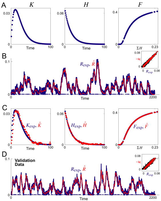
Decoding of noisy synthetic data. As in Fig. 3, but with random noise added to the overall response R_exp before decoding. A noise-free R_exp, for 200 spikes at r = 0.1 in these datasets, was first constructed from the functions K_exp, H_exp, and F_exp in panel A, identical to those in Fig. 3A. In each time bin, a different random number drawn from a Gaussian distribution with zero mean and a given standard deviation was then added to the noise-free R_exp to construct a noisy R_exp (blue curve in panel B). The RMS amplitude of the noise, that is, the RMS difference between the noise-free and noisy R_exp, was computed analogously to the RMS error E_R using the equivalent of Eq. 9. In panel B, the amplitude of the noise was 22.1%. The algorithm then decoded the noisy R_exp to estimate R̂ (red curve in panel B). The inset in panel B plots R̂ against the noisy R_exp (black dots) as well as against the underlying noise-free R_exp (red dots). The error E_R of R̂ relative to the noisy R_exp was 25.2%, but relative to the noise-free R_exp only 12.4%. In panel C, E_K was 31.6%, E_H 9.8%, and E_F 1.7%. For the validation data in panel D, the noise amplitude was 24.1%, E_R relative to the noisy R_exp 24.9%, and E_R relative to the noise-free R_exp 11.9%. Time is in time bins of duration Δt and amplitude is in arbitrary units.