Using Support Vector Machines to Detect Therapeutically Incorrect Measurements by the MiniMed CGMS®

Abstract

Background

Current continuous glucose monitors have limited accuracy mainly in the low range of glucose measurements. This lack of accuracy is a limiting factor in their clinical use and in the development of the so-called artificial pancreas. The ability to detect incorrect readings provided by continuous glucose monitors from raw data and other information supplied by the monitor itself is of utmost clinical importance. In this study, support vector machines (SVMs), a powerful statistical learning technique, were used to detect therapeutically incorrect measurements made by the Medtronic MiniMed CGMS^®.

Methods

Twenty patients were monitored for three days (first day at the hospital and two days at home) using the MiniMed CGMS. After the third day, the monitor data were downloaded to the physician's computer. During the first 12 hours, the patients stayed in the hospital, and blood samples were taken every 15 minutes for two hours after meals and every 30 minutes otherwise. Plasma glucose measurements were interpolated using a cubic method for time synchronization with simultaneous MiniMed CGMS measurements every five minutes, obtaining a total of 2281 samples. A Gaussian SVM classifier trained on the monitor's electrical signal and glucose estimation was tuned and validated using multiple runs of k-fold cross-validation. The classes considered were Clarke error grid zones A+B and C+D+E.

Results

After ten runs of ten-fold cross-validation, an average specificity and sensitivity of 92.74% and 75.49%, respectively, were obtained (see Figure 4). The average correct rate was 91.67%.

Conclusions

Overall, the SVM performed well, in spite of the somewhat low sensitivity. The classifier was able to detect the time intervals when the monitor's glucose profile could not be trusted due to incorrect measurements. As a result, hypoglycemic episodes missed by the monitor were detected.

Introduction

Current continuous glucose monitors (CGMs) have limited accuracy mainly in the low range of glucose measurements. This lack of accuracy is a limiting factor in their clinical use and in the development of the so-called artificial pancreas, i.e., a closed-loop glucose control device that includes insulin pumps and CGMs.^1,2

Several grid-based methods for assessing the accuracy of glucose meters have appeared in the literature and improve upon the classical methods of assessing accuracy (e.g., correlation, linear regression, mean absolute difference, etc.).³ These grid-based methods include the Clarke error grid (CEG),⁴ the Bland-Altman plot,⁵ the consensus grid⁶ and the continuous glucose error-grid analysis.^7,8 These methods are based on a grid in error space representing error significance in terms of therapeutic criteria. Although none of these methods can be considered as the best, the CEG is the one most commonly accepted by the community. The ability to detect incorrect measurements from a CGM, from the information supplied by the monitor itself, is of utmost importance in clinical applications. This detection of errors would facilitate the interpretation of continuous glucose profiles, indicate hypoglycemic states missed by the monitor, and highlight other important discrepancies between the monitor's readings and actual glycemia.

In this study, support vector machines (SVMs), a powerful classification technique, were used to detect therapeutically incorrect measurements made by the MiniMed CGMS^® (Medtronic; Natick, MA). Therapeutically incorrect readings were defined as readings belonging to zones C, D, or E in the CEG, i.e., readings that may induce therapeutically inadequate responses. Henceforth, we will refer to these simply as incorrect measurements. Readings classified in zones A or B in the CEG will be denoted correct measurements. To distinguish between correct and incorrect measurements, an SVM classifier is trained on information provided by the measuring device, such as the monitor's glucose estimation, input signal for glucose (ISIG), and voltage counter transfer ratio (VCTR). While the MiniMed CGMS was used in this proof-of-concept work, the technique itself could be applied to other monitors after adequate training.

This article is organized as follows. First, the clinical, experimental setup for the data acquisition phase and the data conditioning are described. The fault detection problem is transformed into a classification problem and the SVM is motivated. A general introduction about SVMs is given for the unfamiliar reader and the configuration of the classifier used in this work is presented. Next, the experimental results are described. Finally, the most relevant results are highlighted and some conclusions on the applicability of the proposed method are provided.

Methods

Experimental setup

Twenty-two patients with type 1 diabetes mellitus were selected for the study (mean age 27 years with a standard deviation of 5 years; the mean BMI was 24.4 kg/m² with a standard deviation of 2.9 kg/m²; 40% female and 60% male; all patients had diabetes for more than ten years). They also had non-optimal metabolic control, with a hemoglobin A1c greater than 6.5%. Patients were monitored for three days (the first day in the hospital and two days at home) using the MiniMed CGMS MMT-7102. After the third day, monitor data were downloaded to a computer. During the stay in the hospital (12 hours), blood samples were taken every 15 minutes for two hours after meals and every 30 minutes otherwise. Plasma glucose was measured in duplicate by the glucose oxidase method, using a Glucose Analyzer II (Beckman Instruments, Brea, CA), with a coefficient of variation less than 2%. Only monitor data obtained during these 12 hours were used in the analysis. For the other data, no gold standard measurement was available. The subject's usual insulin dosage, including the amount and the administration site, was maintained throughout the study. In addition, food ingestion was maintained with normal meals, although food preparation was supervised by nutrition experts.

Before the start of the study, the patients participated in a training seminar about the MiniMed CGMS and the clinicians assessed their knowledge regarding the functions and use of the device.

During the study, patient 5 met the exclusion criteria defined in the protocol and was withdrawn (anemic state was detected). Data collected from patient 6 was also disregarded because of the detection of a calibration point introduced erroneously in the monitor. Thus, a total of 20 patients were included in the study.

Data conditioning

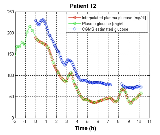
For each of the 20 patients who finished the experiment, 40 plasma glucose readings were obtained. Six measurements were dismissed due to measurement problems, resulting in a total of 794 samples: 97 samples were in the hypoglycemic range (≤70 mg/dl), 352 in hyperglycemic range (>180 mg/dl) and 345 in the euglycemic range. Plasma glucose measurements were interpolated using a cubic method for time synchronization with the simultaneous MiniMed CGMS measurements every five minutes. MATLAB^® release 2006b (The MathWorks, Natick, MA) was used for this purpose. A total of 2281 valid data pairs were obtained. As an example of the data conditioning procedure, the resulting valid data pairs for patient 12 are shown in Figure 1. Application of the CEG to the 2281 data pairs revealed that 94% were located in zone A+B, while 6% were in zone C+D+E.

Figure 4.

Performance of the classifiers obtained in the validation process (ten runs of ten-fold cross-validation) shown on an ROC graph. The average specificity and sensitivity were 92.74% and 75.49%, respectively. TPR, true positive rate; FPR, false positive rate; ROC, receiver operating characteristic.

Figure 1.

Time synchronization of a continuous glucose monitoring system and plasma glucose values by cubic interpolation for patient 12. Blue circles correspond to the MiniMed CGMS^® measurements every five minutes; green circles correspond to plasma measurements obtained every 15 minutes for two hours after a meal and every 30 minutes otherwise; red circles correspond to interpolated plasma glucose values synchronized with the CGMS measurements. Time zero represents the instant at which the monitor started supplying readings (approximately two hours after the start-up of the monitor). A gap in the data supplied by the monitor happened approximately between hours seven and eight.

Support Vector Machines

Support Vector Machines are a well-established technique in statistical learning theory used for classification and regression,⁹ offering excellent performance especially when applied to complex real-world problems that may be difficult to analyze theoretically. Classification of the problem consists of assigning a class label to data points in input space (e.g., class A and B). All data points in the same class express the same pattern to be learned.

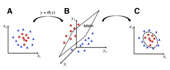
In the context of this paper, this corresponds to incorrect and correct measurements made by the monitor. If a line (i.e., a hyperplane) can be defined separating class A and B data points, then it is a linear classification problem. However, in complex problems, the boundary separating the two classes is nonlinear. SVMs are capable of tackling nonlinear classification very efficiently. This is carried out by transforming the input space, x, into a new higher-dimensional space (the feature space) using nonlinear mapping, y = θ(x), where a linear classification is carried out. Thus, SVMs calculate linear boundaries in an extended space to represent nonlinear boundaries in the original space (see Figure 2).

Figure 2.

Illustration of the support vector machine (SVM), a nonlinear classification technique. The original input space (A) is extended through a non-linear mapping [indirectly defined by the selection of the kernel function; (B)]. Then, linear classification is carried out (C). The linear boundary in the extended space induces the non-linear boundary in the original space.

Linear classification is carried out by computing the maximum margin hyperplane (MMH) in the feature space. This hyperplane is calculated so that the maximum possible margin is left between elements of the different classes. This corresponds to a quadratic programming problem, with a unique solution corresponding to a linear combination of a subset of the training data points, called support vectors.^10,11

The information required to compute the MMH is the inner product of the transformed data K(x,x′): = θ(x) · θ(x′). In some cases, the kernel K can be computed directly from the input data, without explicit knowledge of the nonlinear transformation θ. The selection of the kernel function will indirectly define the feature space. This makes these kernel functions efficient, so that they are widely used. Typical kernel functions are:

• Degree d polynomial: $K\left(x,x^{\prime }\right)={\left(x\cdot x^{\prime }+1\right)}^d$

• Gaussian radial basis function: $K\left(x,x^{\prime }\right)=\exp \left(-\frac{{\Vert x\cdot x^{\prime }\Vert }^2}{2{\sigma }^2}\right)$

• Sigmoidal: $K\left(x,x^{\prime }\right)=\tanh \left(\varkappa x\cdot x^{\prime }+\delta \right)$

The kernel selected also determines the shape of the nonlinear boundary, which is a weighted sum of kernel function evaluations. These weights have to be learned through training data. SVM training involves minimizing training errors (empirical risk) and the probability of incorrectly classifying unknown data (structural risk). SVMs have been successfully applied in biomedical engineering to support diagnostics and therapeutics with excellent results in cancer diagnosis¹² or idiopathic scoliosis.¹³

In this study, an SVM classifier with a Gaussian radial basis kernel was tuned and validated using k-fold cross-validation (k = 10) ten times (a total of 100 problems solved). At each ten-fold cross-validation, the data were randomly partitioned into ten approximately equal, disjointed sets using the Bioinformatics Toolbox™ in MATLAB release 2006b.

The classes considered in the classification problem were the CEG zones A+B (correct measurements) and C+D+E (incorrect measurements).

The features vector $X=(ISIG,\frac{dISIG}{dt},\hspace{0.17em}\hspace{0.17em}VCTR,\hspace{0.17em}\hspace{0.17em}{G}_{CGMS})$ represented the electrical characteristics of the measured signal and the MiniMed CGMS estimation algorithm. This features vector was considered and normalized by its Euclidean norm $\sqrt{X^T\hspace{0.17em}X}$. ISIG represents the sensor current, dISIG/dt its derivative with respect to time, VCTR the registered voltage, and G_CGMS the glucose estimation provided as output from the MiniMed CGMS monitor. Finally, to avoid high dimensionality and reduce computational time, the projection onto the ISIG and VCTR dimensions was used as the input data set.

Classification of training data was performed using the CEG with interpolated plasma glucose values as the gold standard. It is important to provide the classifier with incorrect measurements during the training phase so that their patterns can be learned. As stated earlier, data from the first day (inpatient period) were used in the study because only during that time were gold standard measurements available for validation. This corresponds to the time of the poorest performance of the monitor and thus more errors are expected. Once trained, the classifier will detect incorrect measurements, regardless of the day.

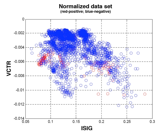
Henceforth, a “negative” result will refer to a data point falling in zones A or B while a “positive” result will refer to data points falling in zones C, D or E. Figure 3 shows the classification of the whole data set. As can be observed, both positive and negative data points are not linearly separable in the VCTR-ISIG space. However, some grouping is observed. Thus, an SVM is ideal for solving the complex problem of separating the classes through a nonlinear transformation into a higher dimensional space where then, finally, the classes can be separated.

Figure 3.

Projected normalized data set. Positive class (in red) corresponds to CEG zones C+D+E and negative class (in blue) to zones A+B.

Tuning of the Gaussian SVM was performed iteratively until satisfactory results were obtained using the Bioinformatics Toolbox in MATLAB release 2006b.

Results

After ten runs of ten-fold cross-validation, an average specificity and sensitivity of 92.74% and 75.49%, respectively, were obtained (see Figure 4). The average correct rate was 91.67%. Thus, the classifier exhibited an excellent specificity, which implies that correct measurements from the monitor are captured well by the system. A wider range of sensitivities was observed among the different runs during cross-validation. Although in some cases the value obtained was low (i.e. there were a significant number of false positives), performance should be evaluated from the perspective of glucose profiles rather than individual samples. Such an analysis is presented in the Discussion section.

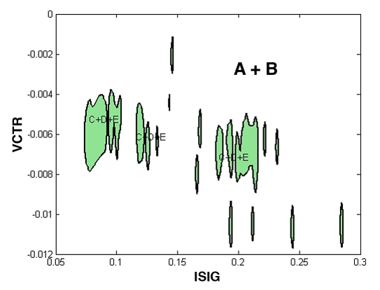
To illustrate the expected performance, one sample classifier was selected out of the set of 100. This classifier had a 92.49% specificity, 73.33% sensitivity, and 91.23% correct rate, similar to the average performance of the whole set. Figure 5 shows the regions obtained in this case for the C+D+E class (closed filled regions) and A+B class (the complementary set). Incorrect measurements are concentrated in three principal areas and a small set of dispersed areas.

Figure 5.

Classification regions obtained for classes A+B and C+D+E for an average classifier.

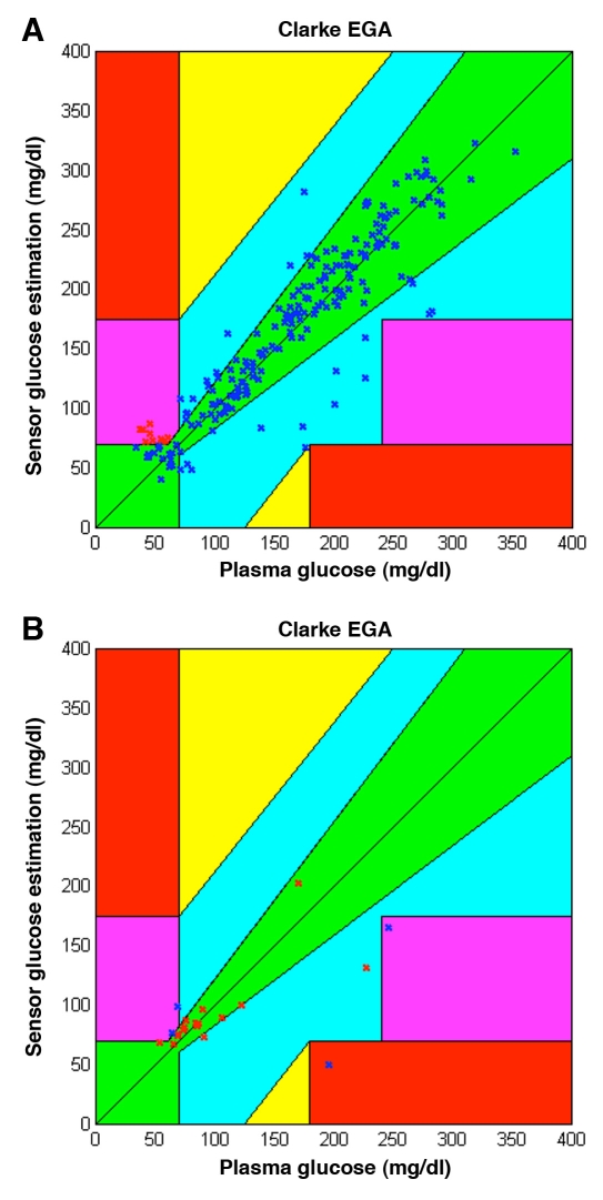
Classification results for the test data (228 samples) from this sample classifier are shown in Figure 6. In Figure 6A the correctly classified data pairs are shown on the CEG. They comprise both incorrect (true positive) and correct (true negative) measurements. Incorrect measurements only appear in CEG zone D, while no point is located in zones C and E. Correctly classified data points are thus located in zones A, B, and D. On the other hand, Figure 6B presents all misclassified points, including incorrect (false positive) and correct (false negative) measurements. In this case, misclassified points appear in zones A, B, D, and E.

Figure 6.

Classifications carried out by the sample (average) classifier for the test data. (A) True positives are shown with red Xs and true negatives with blue Xs. (B) False negatives are shown with red Xs and false positives with blue Xs.

From Figure 6 it can be observed that the percentage of misclassifications is low. For this specific trial, 91.23% of the test points were classified correctly. From a total of 15 incorrect measurements by the monitor, four were misclassified and thus undetected by the system; thus 73.33% of the incorrect measurements were detected. Sixteen of 213 (7.5%) correct measurements were misclassified and reported as incorrect measurements.

Discussion

The results of this study indicate that, on average, the classifier exhibits a very good specificity (92.74%), which implies that correct measurements from the monitor will be captured accurately. A wider range of sensitivities was observed among the different runs carried out during cross-validation, with an average of 75.49%. A sensitivity value that is too low implies that a significant number of false negatives may appear. This was seen in the performance of the sample classifier described earlier. With this classifier 26.67% of the incorrect measurements in the validation data set remained undetected.

To determine the extent to which sensitivity and specificity influence global performance, an analysis must be performed in terms of glucose profiles rather than individual samples. The performance may be considered good if the system is able to detect the time intervals when the profile should not be trusted because of incorrect measurements with clinical consequences, such as untreated hypoglycemic episodes.

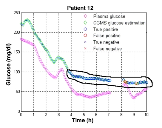
Thus, to determine the influence of sensitivity and specificity, individual glucose-time profiles given by the monitor were classified using the sample classifier described earlier. Figure 7 shows the results for one patient when missed hypoglycemic episodes occurred. Magenta diamonds represent the gold standard and green diamonds the measurements of the MiniMed CGMS. Within the green diamonds, a blue marker indicates a correctly classified sample (an “X” stands for a sample classified as A+B and a circle represents a sample classified as C+D+E); a red color indicates a misclassified sample. Figure 7 shows that hypoglycemia remained undetected by the monitor from approximately hour 4 onward. This fact is correctly detected by the classifier (denoted by the blue circles). Although some false negatives appear (red circles), they do not interfere with the general conclusions drawn from the graph.

Figure 7.

Detection of missed hypoglycemia. In patient 12, incorrect measurements (encircled in black) from the MiniMed CGMS^® were detected from approximately hour four onward, by the electrical signal of the monitor and its glucose estimation. Glucose measurements performed on collected plasma indicated that the patient was in a hypoglycemic state while the monitor reported a value in the euglycemic range. No error was raised by the monitor, except during the displayed data gap, where a calibration error (CalErr) was recorded.

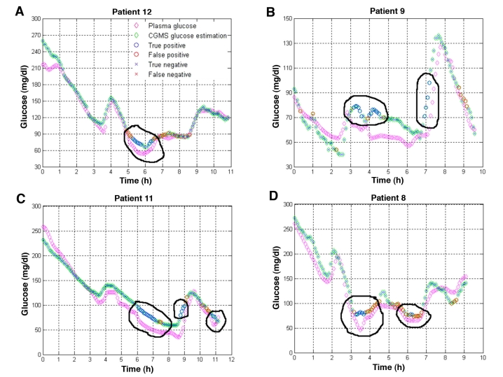
Figure 8 shows the results for the rest of the patients when hypoglycemic episodes remained undetected by CGMS^®. In most cases, hypoglycemia occurred around 5:00 p.m. (approximately six hours after the monitor started supplying data). In Spain, lunch is usually eaten at approximately 2:00 p.m., so 5:00 p.m. falls between lunch and dinner, when most patients are prone to hypoglycemia. No specific calibration was done at that time. In all cases, the classifier detected these episodes from the electrical signal and MiniMed CGMS glucose estimations. Although a significant number of misclassifications occurred in some patients (see Figure 8D, for example), these misclassifications did not have a significant impact on the analysis of the profiles, except in overestimating the duration of the hypoglycemic episodes.

Figure 8.

Examples of detection of missed hypoglycemic episodes (encircled in black) in four patients. (A) In patient 21, missed hypoglycemia was detected, however, the classifier overestimated its duration. (B) In patient 9, missed hypoglycemia was correctly detected. Appearance of false negatives was negligible, except during a short period in the final downward trend in glycemia, where consecutive misclassifications appeared. (C) In patient 11, missed hypoglycemia (in this case due to the lag between plasma and interstitial glucose) was correctly detected by the classifier. Misclassifications did not interfere with the main conclusions. (D) In patient 8, the number of misclassifications was higher than in the other patients, however, the missed hypoglycemia between the hours of three and four was detected by the classifier. The same happened with the episode of mild hypoglycemia near hour six.

This analysis concluded that SVM classifiers can be used to detect therapeutically incorrect measurements provided by the MiniMed CGMS. For all patients, missed hypoglycemic states and other incorrect measurements, as defined by the CEG, were detected. The presence of false positives did not alter the conclusions drawn from the analysis of time profiles.

The SVM can thus support the clinician in the interpretation of readings from CGMs. While this study focused on the MiniMed CGMS, which is a retrospective monitor, the method could also be applied, with appropriate training, to real-time monitors. These alternative applications would require data only on the corresponding monitor's electrical signal and glucose estimation. However, further research is needed to confirm the general applicability of the SVM to glucose monitors.

Future research might include the investigation of other tests, such as the consensus grid and continuous glucose error-grid analysis for the definition of classes and the reconstruction of glucose profiles once incorrect estimations have been detected. Applications to real-time monitors may also be investigated.

Abbreviations

CEG

Clarke error grid

CGM

continuous glucose monitor

ISIG

input signal for glucose

MMH

maximum margin hyperplane

SVM

support vector machine

VCTR

voltage counter transfer ratio

Funding

This work was supported in part by the Spanish government under the grants DPI-2004-07167-C02-01, DPI-2004-07167-C02-02, DPI-2007-66728-C02-01 and DPI-2007-66728-C02-02 and by the European Union through FEDER funds.

References

- 1.Mazze RS. Making sense of glucose monitoring technologies: from SMBG to CGM. Diabetes Technol Ther. 2005;7(5):784–787. doi: 10.1089/dia.2005.7.784. [DOI] [PubMed] [Google Scholar]
- 2.Guerci B, Floriot M, Böhme P, Durain D, Benichou M, Jelliman S, Drouin P. Clinical performance of CGMS in type 1 diabetic patients treated by continuous subcutaneous insulin infusion using insulin analogs. Diabetes Care. 2003;26(3):582–589. doi: 10.2337/diacare.26.3.582. [DOI] [PubMed] [Google Scholar]
- 3.Wenholt IM, Hoekstra JB, Devries JH. A critical appraisal of the continuous glucose–error grid analysis. Diabetes Care. 2006;29(8):1805–1811. doi: 10.2337/dc06-0079. [DOI] [PubMed] [Google Scholar]
- 4.Clarke WL, Cox D, Gonder-Frederick LA, Carter W, Pohl SL. Evaluating clinical accuracy of systems for self-monitoring of blood glucose. Diabetes Care. 1987;10(5):622–628. doi: 10.2337/diacare.10.5.622. [DOI] [PubMed] [Google Scholar]
- 5.Bland JM, Altman DG. Statistical methods for assessing agreement between two methods of clinical measurement. Lancet. 1986;1(8476):307–310. [PubMed] [Google Scholar]
- 6.Parkes JL, Slatin SL, Pardo S, Ginsberg BH. A new consensus error grid to evaluate the clinical significance of inaccuracies in the measurement of blood glucose. Diabetes Care. 2000;23(8):1143–1148. doi: 10.2337/diacare.23.8.1143. [DOI] [PubMed] [Google Scholar]
- 7.Kovatchev BP, Gonder-Frederick LA, Cox DJ, Clarke WL. Evaluating the accuracy of continuous glucose-monitoring sensors: continuous glucose-error grid analysis illustrated by TheraSense Freestyle Navigator data. Diabetes Care. 2004;27(8):1922–1928. doi: 10.2337/diacare.27.8.1922. [DOI] [PubMed] [Google Scholar]
- 8.Clarke WL, Anderson S, Farhy L, Breton M, Gonder-Frederick L, Cox D, Kovatchev B. Evaluating the clinical accuracy of two continuous glucose sensors using continuous glucose-error grid analysis. Diabetes Care. 2005;28(10):2412–2417. doi: 10.2337/diacare.28.10.2412. [DOI] [PubMed] [Google Scholar]
- 9.Hearst MA. Support Vector Machines. IEEE Intelligent Systems. 1998;13(4):18–28. [Google Scholar]
- 10.Hastie T, Tibshirani R, Friedman J. The elements of statistical learning: data mining inference, and prediction. New York: Springer; 2001. [Google Scholar]
- 11.Vapnik VN. The nature of statistical learning theory. New York: Springer-Verlag; 1995. [Google Scholar]
- 12.Chuan Lu, Devos A, Suykens JAK, Arus C, Van Huffel S. Bagging linear sparse Bayesian learning models for variable selection in cancer diagnosis. IEEE Trans Inf Technol Biomed. 2007;11(3):338–347. doi: 10.1109/titb.2006.889702. [DOI] [PubMed] [Google Scholar]
- 13.Ramirez L, Durdle NG, Raso VJ, Hill DL. A support vector machines classifier to assess the severity of idiopathic scoliosis from surface topography. IEEE Trans Inf Technol Biomed. 2006;10(1):84–91. doi: 10.1109/titb.2005.855526. [DOI] [PubMed] [Google Scholar]