Abstract
Clustering and correlation analysis techniques have become popular tools for the analysis of data produced by metabolomics experiments. The results obtained from these approaches provide an overview of the interactions between objects of interest. Often in these experiments, one is more interested in information about the nature of these relationships, e.g., cause-effect relationships, than in the actual strength of the interactions. Finding such relationships is of crucial importance as most biological processes can only be understood in this way. Bayesian networks allow representation of these cause-effect relationships among variables of interest in terms of whether and how they influence each other given that a third, possibly empty, group of variables is known. This technique also allows the incorporation of prior knowledge as established from the literature or from biologists. The representation as a directed graph of these relationship is highly intuitive and helps to understand these processes. This paper describes how constraint-based Bayesian networks can be applied to metabolomics data and can be used to uncover the important pathways which play a significant role in the ripening of fresh tomatoes. We also show here how this methods of reconstructing pathways is intuitive and performs better than classical techniques. Methods for learning Bayesian network models are powerful tools for the analysis of data of the magnitude as generated by metabolomics experiments. It allows one to model cause-effect relationships and helps in understanding the underlying processes.
Electronic supplementary material
The online version of this article (doi:10.1007/s11306-009-0166-2) contains supplementary material, which is available to authorized users.
Keywords: Constraint-based learning, Bayesian networks, Metabolic pathways, Tomato volatiles, oxylipin pathway, urea/citric acid cycles
Introduction
Metabolomics plays an increasingly important role in the research area of drug discovery, food & nutrition, plant and animal biology and many other applications. Where transcriptomic and proteomic analysis does not tell the complete story, metabolic profiling can add significantly to the picture of what is happening inside a living cell. Statistical and mathematical techniques are commonly used to correlate changes in metabolic composition with changes in biological conditions (Suizdak 2003; Eiceman and Karpas 2005; Gohlke 1959; Weckwerth 2003; Kopka et al. 2004). Chromatography coupled to mass spectrometry based methods, e.g., GC-MS and LC-MS, have been the most popular metabolic profiling techniques over the past decade. Hundreds of new metabolites have been identified in plants (Fiehn et al. 2000; Moco et al. 2006; Schauer et al. 2006) and the improved sensitivity of modern methods has led to an increased amount of metabolic information. Techniques such as these have enabled identification of metabolites at much higher resolutions than previously possible. Interesting relationships can thus be found by integrating different types of data (omics) from various analytical sources. In this paper, Bayesian network learning methods are explored to uncover molecular pathways of tomato metabolism. This is done by using constraint-based learning methods. The related research is reviewed in the next section.
Related research
Various methods in classical multivariate statistics have been used in the past to discover and visualize complex metabolic networks using supervised and unsupervised clustering methods. Clustering techniques (Opgen-Rhein and Strimmer 2007) provide good summarization of data concerning functional relations between metabolites but as these methods are global one cannot expect to find relations which are relevant for small subsets of data. These techniques are good for capturing whether or not variables influence each other; however the nature of interaction between metabolites is complex and cannot be estimated using only linear correlations (Husmeier et al. 2005). Furthermore, domain knowledge, which often plays a vital role to find novel relationships and which can be obtained from literature and experts, cannot be incorporated in these traditional techniques with the exception of choosing the proper parametric form of the functional interaction between variables, e.g., linear or exponential. Learning logistic regression models from data is the standard approach for capturing the statistical interactions among a set of input variables to predict the value of a dependent, or output, variable. However, it is difficult to establish the impact of process changes among the variables using only regression models. Moreover, when there are insufficient data it cannot accommodate background knowledge (expert judgement) and causal explanation to the relationships obtained.
We present here a constraint-based Bayesian network approach, which is a specialized form of graphical models (Jordan 2004). Use of Bayesian networks to analyze biological datasets in various genomics domain has been growing in the last decade. Different types of Bayesian network learning methods, e.g., search and score, have been used to recover target-regulator pairs from a yeast cell cycle microarray datasets (Murphy 2002); Zou and Conzen 2005), and also significant work has been done by Friedman et al. to reconstruct gene regulatory networks from microarray datasets (Friedman et al. 2000). Similar techniques have also been used for pathway identification to understand the underlying biological processes. In this paper we demonstrate how Bayesian network learning techniques can be used to uncover a very important metabolic pathway (oxylipin pathway) which plays an important role in the ripening of fresh tomatoes. We also show why this technique is better than other statistical techniques used in this domain.
In principle a Bayesian network is a graphical representation of a multivariate probability distribution and is an example of a probabilistic network. A probabilistic network typically consists of nodes connected by edges, where each node corresponds to a random variable and edges represent dependence between them. Absence of edges between nodes represents conditional independence. Bayesian networks, a special type of a probabilistic network, contain directed edges, also called as arcs or arrows. The advantage of Bayesian networks over alternative techniques (e.g., logistic regression) is that they allow explicit representation of the mutual interactions among variables and groups of variables. They take into account the explanatory power of known variables in an intuitively simple graphical format. As a Bayesian network is a multivariate probability distribution with statistical independence assumptions, it is possible to reason probabilistically with this representation (For an example see the next section). The other advantage lies in the fact that probability distributions can be updated in the light of new, known information. This is why Bayesian networks can be used to support decision making. The results obtained using this technique are exceptionally intuitive and this type of analysis is not possible by classical analysis tools. Nonetheless, there are a few limitations; for example when the number of variables increases in size the computational complexity increases, which is NP-hard. Apart from this, Bayesian networks, like regression models, are also sensitive to sample size. However, on the positive side most biological processes are hierarchical in nature and there are more variables then relationships between them i.e., the graphs are sparse.
Example
In Fig. 1 we present an example of the urea and citric acid cycles. These two cycles are linked by the synthesis of fumarate. To highlight the basics of the Bayesian network method, the reactions leading to and from fumarate are shown in Fig. 2, where both the probability distribution and the graph are shown. The graph encodes rather subtle information about statistical dependence and independence between sets of variables. For example, according to the graph in Fig. 2, the concentrations of both argininosuccinate and succinate are independent as there are no arrows connecting these nodes. Both production of fumarate and malate are a common consequence of presence of argininosuccinate and succinate (as there are directed paths going from these nodes to both fumarate and malate). The semantics attached to Bayesian networks implies that if either fumarate or malate or oxaloacetate are observed in high levels, then argininosuccinate and succinate become dependent given the fact that we know levels of fumarate. Finally, argininosuccinate (or succinate) and oxaloacetate are conditionally independent given the concentration levels of fumarate. It also means that if one has observed high or low levels of fumarate then this does not convey any new information about concentrations of malate or oxaloacetate, and vice versa. Given a Bayesian network, any conditional probability involving any of the variables included in the model can be computed.
Fig. 1.
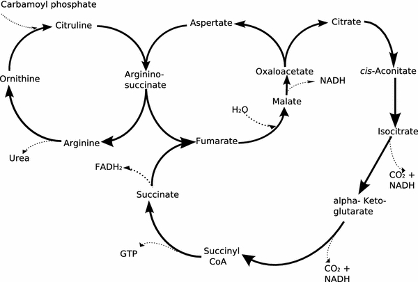
Urea/Citric Acid cycle
Fig. 2.
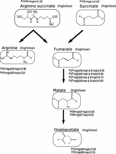
Example of a simple Bayesian network consisting of a probability distribution Pr and a directed graph. The probability distribution Pr is specified using conditional probability distribution associated to the individual nodes, such as Pr(A = high · AS = high) = 0.96
It is a standard practice to compute probabilities of individual variables from a set of variables. These probabilities are referred as marginal or conditional and are updated by fixing observations over one or more variables.
Figure 3 shows the bar graphs associated with the individual variables when the frequency of states of these variables are computed; in Fig. 4 the variables have been conditioned on the assumption that oxaloacetate=high to display that for the case when the concentration is higher for a certain metabolite. In both figures simply looking at the shape of the bar graphs already conveys much information on the concentration levels of each metabolite.
Fig. 3.
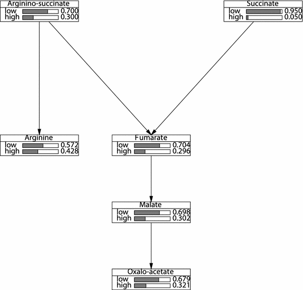
Prior marginal probability distributions for the Bayesian belief network shown in Fig. 2
Fig. 4.
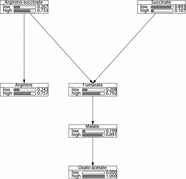
Posterior marginal probability distributions for the Bayesian belief network after entering evidence on concentration levels of oxaloacetate. Note the increase in probabilities of the levels of concentrations of both oxaloacetate and argininosuccinate compared to Fig. 3. It also predicts that it is more likely that the %concentration levels of argininosuccinate to be high
Overview of Bayesian networks
Bayesian networks can be learned from data as a standard practice in multivariate statistics, but as they are easily understood they can also be manually constructed based on expert knowledge in a particular problem domain. For example, if one knows the interaction of metabolites in a certain pathway, one can even make a hypothetical network based on literature without data. Each of the metabolites in the network would be associated with a probability embedded in a contingency table (also known as a conditional probability table), expressing an expert’s degree of belief. As was illustrated above, if one has observed a level of one or more compounds it is possible, using the Bayesian network, to predict the likelihood or concentration levels of the other compounds. Thus the likelihood represents the concentration levels of metabolites. The important aspects of understanding Bayesian networks lies in the fact that the graph structure of network is separate from the probability distribution associated with it.
The graphical nature of the network combined with probability theory allows one to do data analysis in an intuitive way. It is important to understand the interaction between different variables but it is more important to understand the nature of these relationships. From example in the previous section representing urea/citric acid cycle in Fig. 1 argininosuccinate, fumarate and malate represent a serial connection, arginine, argininosuccinate and fumarate represent a diverging connection and argininosuccinate, fumarate and succinate represent a converging connection. As mentioned before knowing information about the concentrations levels of fumarate makes argininosuccinate and malate independent in a serial connection, knowing concentration levels of argininosuccinate make arginine and fumarate independent in a diverging connection and knowing concentration levels of fumarate makes argininosuccinate and succinate dependent in a converging connection.
Formally, a Bayesian network represents an acyclic directed graph (ADG), i.e., a set of nodes, or vertices, and directed edges, or arcs, and is defined as a pair G = (V,E), where V is a finite set of distinct nodes and  is a set of distinct arcs. A pair
  is denoted by an arc u → v from u to v and it is said that u is a parent of v and v is said to be a child of u, often this relationship also represents a cause-effect relationship. A path
  is a set of distinct nodes such that v
i → v
i+1 or v
i ← v
i+1, for each i. A path is called directed if v
i ← v
i+1 or v
i → v
i+1, for each i. A node v is called a descendant of a node u if there is a directed path from u to v in the graph. Statements on conditional dependence and independence can be derived from the graph using the d-separation
criterion (Pearl 1998). The basic idea of d-seperation is that just by looking at the graph it is possible to derive independence information about the associated probability distribution of a Bayesian network. Consider Fig. 5, which depicts three types of subgraphs which are relevant in interpreting a Bayesian network. The subgraphs X → Y → Z and X ← Y ← Z, called serial connection and X ← Y → Z, called diverging connection, are equivalent. Then there is also the non-equivalent converging connection. All three of these causal situations give rise to different conditional independence of the associated random. Formally d-separation is expressed as follows: Two nodes on an ADG, G = (V,E) are said to be d-separated by a set of nodes
  if there is a node w such that either:
 and w does not have a converging connection on any path connecting the nodes and w is on this path, or
 and neither any of the descendants of w in S.
Fig. 5.
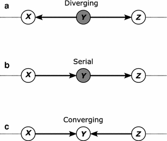
Three different graph structures of a Bayesian network and their interpretation
If two variables are d-separated given a set of variables S in a directed graph, then they are conditionally independent given another set of variables in all probability distributions compatible with the graph. Two variables X and Y are conditionally independent given a set of variables S if knowledge on X gives no additional information on Y once we know about S.
Bayesian networks are also said to be an independence map, or I-map for short, as independencies can be read off by d-separation from the graph and these also hold for the underlying probability distribution. This property allows us to find independence between variables of interest in a problem domain. d-Separation in a graph structure G is represented by ⫫G and conditional independence in a probability distribution, by ⫫P. Some standard notations used in the context are as follows:
u ⫫G v ∣ S :
 and
and  are d-separated in graph G = (V,E), given a set of nodes W.
U ⫫G V ∣ W : Each
 and each
  is d-separated in graph
  or U and V are d-separated in G, given the set of nodes W.
U
 G
V ∣ W : Each
  and each
  is d-connected, given the set of nodes W.
X ⫫P Y ∣ S : X and Y are conditionally independent given S.
X
 P
Y ∣ S : X and Y are conditionally dependent given S.
P
Y ∣ S : X and Y are conditionally dependent given S.if S = ϕ, and X ⫫P Y ∣ ϕholds, then sets X and Y are called marginally independent.
Not always we will have knowledge about relationships between metabolites of interest in which case we would want to find these relationships from available experimental data. This approach is not uncommon when the number of variables is large and there is little or no knowledge available of the underlying process. Moreover, it can be a laborious task to construct networks of several hundred nodes just by hand. Therefore there has been considerable research in this area to do unsupervised learning of conditional dependence and independence relationships from data. The key assumptions used for this approach are that biological processes are hierarchical in nature and links between metabolites in metabolic processes are sparse in nature. In the past, correlation and clustering methods have been used successfully to identify groups of metabolites clustering together and reconstruct pathways (Yilmaz 2001; Ursem et al. (2008)). Bayesian networks allows us to model causal relationships by looking at the direction of the arrows in the directed graph. Causal relationships play a vital role when we want to find out when one variable causes a change in another variable. Often these relations are investigated by experimental research to determine if changes in one variable truly cause change in another variable. However to generate an equivalent network is still possible using Bayesian network. For Bayesian networks there is the restriction that arrows are not allowed to form directed cycles (paths that end at the node where they started)–these graphs are called acyclic. Of course, there can be feedback loops involved in a problem domain which can be perfectly modeled using another type of Bayesian networks, so-called dynamic Bayesian networks (Murphy 2002), which require time-series data.
Learning in Bayesian networks
Learning the graph of a Bayesian network is done by exploring data using partial correlations as a means to distinguish dependent from independent relationships. To put it simple, direct and indirect relationships can be identified easily from the constructed networks: metabolites missing arrows indicate (conditional) independence. There are two aspects of representing data using this technique viz. qualitative and quantitative. The qualitative aspect includes representation of data using nodes and arrows and these relationships can be quantified using a conditional probability distribution. Constraint-based methods have the advantage that they allow incorporation of prior biological knowledge about dependence of variables, and therefore this has been taken as the method of choice for the present research. We consider here the PC-algorithm (Peter and Clark) (Sprites et al. 2000) which is a constraint-based method. There are certain assumptions to this approach such as the independence between nodes has a perfect representation by an ADG; under this assumption the PC algorithm will discover an equivalent Bayesian network. Another assumption is that networks are sparse, i.e., have few relationships between metabolites as shown in Fig. 1. There are several ways to verify conditional independence relationships which include reducing size of the database, finding correlations, direct query from experts and finding clusters in a causal network.
The algorithm is based on asking true independence relationship between sets of variables of the form X i⫫X j∣S, where S is a subset of variables. An overview of the steps are as follows:
Construct an undirected graph.
Find converging connections, by testing for independence and
Give directions to the links without producing cycles.
Here we consider an imaginary oracle as our expert which tells us if two nodes are conditionally independent given a subset of nodes S (later this oracle will be replaced by statistical test to find partial correlations, e.g., G 2 test or Fisher’s Z transformation). If the oracle (domain expert) says two nodes are conditionally independent given a third node S then we remove the edge between two nodes and make them independent. Asking questions like this for all the nodes involved and recursively deleting edges between nodes based on the answers will result in an undirected graph also known as the skeleton of the network. The next step then is to give directions to the edges based on rules (Meek 1995b) to generate a ADG, sometime there might exist bi-directional arrows which is not a part of Bayesian networks, but its presence indicate hidden nodes, which might have been missed from the experiment or not being observed.
In this paper, we demonstrate how learning and reasoning with Bayesian networks can be used to reconstruct the oxylipin pathway found in the synthesis of fresh tomato volatiles. We show how the results obtained by running Bayesian network analysis on experimental data of biochemical compounds of beef, round and cherry tomatoes supports the elucidation of the nature of the biological processes. For brevity, our focus is only on learning of structures and not on parameter estimation, which is often used to learn the probability distribution of the dataset. Subsequently, we discuss how to interpret the graphs generated by Bayesian network learning (which is an important aspect of data analysis). Prior knowledge obtained from literature is also taken into account in the form of metabolite selection for the analysis. The dataset used includes data of tomato volatile metabolite profiling, as described in (Tikunov et al. 2005). A detailed description of this dataset can be found below in the materials sections of the article.
Materials and methods
Description of the metabolite dataset
Flavors in tomatoes are important targets for plant breeders to improve the quality of fresh tomatoes. Therefore it has become a popular area of research among molecular biologists to study the pathways involved in biosynthesis, of the oxylipin (lipoxygenase) pathway of volatile compounds (VOC, volatiles) in tomatoes. In plants the substrates of these pathways are linoleic and linolenic acid, while their mammalian equivalents are arachidonic and eicosapentaenoic acids. Tomato volatiles are generally divided into six groups (Yilmaz 2001) lipid derived, carotenoid related, amino acid related, terpenoids, lignin related and miscellaneous. Each group participates in different pathways involved in the biosynthesis of the aroma volatiles. Figure 6 shows formation of lipid-derived volatiles through one of these pathways. There has been substantial research in this area, however the exact nature of the relationship between volatile compounds involved is still unknown.
Fig. 6.
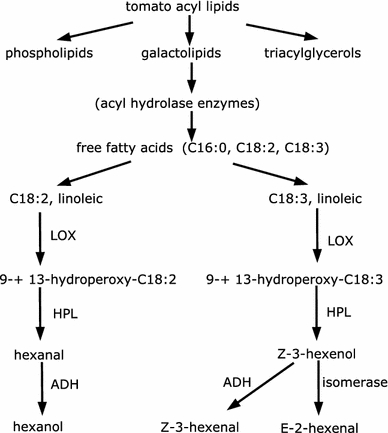
Formation of lipid-derived volatiles through biosynthesis in the oxylipin pathway
Volatiles have been analyzed using gas chromatography mass spectrometry in ripe fruits of 94 tomato (Solanum lycopersicum L.) varieties as described in Tikunov et al. (Tikunov et al. 2005). The varieties selected represent a considerable collection of genetic and therefore phenotypic variation. 322 VOC have been detected and 69 VOC identified most reliably have been chosen for the present study. This set of 69 VOC contains metabolites of 7 biochemical groups: volatiles derived from lipids, two phenylalanine derived groups, leucine and/or isoleucine derived volatiles, open-chain carotenoid derivatives, cyclic carotenoid derivatives and terpenoids. The last three groups are biochemically related and called isoprenoids.
Analysis
We consider here finding relationships between volatile metabolites of lipid derivatives involved in the oxylipin/lipoxygenase (LOX) pathway which occurs during ripening of tomato fruit (Yilmaz 2001) as depicted in Fig. 6. We used the package pcalg (Kalisch and Buhlmann 2007) which is an implementation of the PC algorithm in R (R Development Core Team 2008) which is an open source environment for statistical computing to perform the analysis on a real-life dataset as mentioned in the Sect. 3 of the article. The inputs were the tomato dataset and the algorithm allows to set a threshold to find significant conditional (independent) relationships between these metabolites. The algorithm generates a graph object which is an ADG. A bidirectional arrow in such network implies presence of hidden variables from the experiment being conducted (hidden factors or latent variables), e.g., when a metabolite is missing from the experiment (Beal et al. 2005). Here we show how this algorithm performs on a real-life dataset and finds relationships among metabolites of interest which are biologically meaningful and by taking into account the prior knowledge the generated network is compared to the established knowledge found in literature. This can be done by counting missing edges (false negatives) and extra edges (false positives) which were computed for these metabolites by the algorithm. Finally the structure Hamming distance metric (Tsamardinos et al. 2006) a measure to calculate the number of substitutions required to transform one graph to another, is used to calculate the distance (difference) of the computed network from the actual network (pathway). The lower this score is, the better the PC algorithm has performed on the dataset.
The visualization of complex networks is not easy and the knowledge represented by them is sometimes not obvious just by looking at these complex networks. The key to solving these issues is to make use of an interactive graph which allows looking at the chemical structures and getting relevant information from online repositories using well-established visualization techniques. We therefore implemented a framework which handles these issues, and the networks shown in this paper have been created using the tools. The tool was developed using open source software and standards, such as Graphviz (http://www.graphviz.org) and SVG(http://www.w3.org/Graphics/SVG/). All the scripts used for construction of networks are available from the authors upon request.
Results and discussion
A primary interest in biology is finding novel biochemical pathways describing relationships between metabolites and their dependence on environmental factors. Often the data arising from experiments are not completely observed; this scenario is represented as “data being incomplete and the structure of the Bayesian network being unknown”. Clearly, this is also the most difficult case from a computational point of view. Incomplete data may involve missing values, and imputation techniques are employed to find appropriate values; these values are assumed to be missing at random. Sometimes particular crucial variables are missing, called hidden or latent variables. Using optimization algorithms such as the Expectation Maximization(EM) algorithm, it is sometimes possible to learn all parameters, including the hidden ones (Dellaert 2002 & Elidan and Friedman 2003).
In this study we show how parts of a plant metabolic system can be reconstructed and visualized by applying Bayesian networks. We focused on 69 volatile compounds and the choice of these metabolites was based upon prior knowledge obtained from the domain experts and relevant literature (Tikunov et al. 2005; Yilmaz 2001; Yilmaz et al. 2001). We used constraint-based learning of Bayesian networks with a very low significance level α of 0.0001 on this dataset. The test statistic used to find the relationship and their strength are based on Fisher’s Z transformation (Kalisch and Buhlmann 2007). A Bayesian network estimates a ADG and so relationships do not form a cycle, observing all such relationships indicate hidden variables which might have been missed by chance or not being observed in the experiment. As Bayesian networks generate equivalent structures, considering the example from Fig. 5, subgraphs A → B → C, A ← B ← C and A ← B → C are equivalent. Therefore the methods described in the analysis section estimated 13 arcs; when comparing this estimated network with the relationships found in the literature we were able to find 66 % true positives, 7 % false positives and a structure Hamming distance of 9, meaning that it would take 9 operations of adding, deleting and changing the direction of arrows to reach the true graph. Analysis of the experiment using the search-and-score (Heckerman 1995) method produced a graph with 16 arcs, and contained only 25% true positives and 56% false positives (the corresponding network graph can be found in the supplementary material) and a structure Hamming distance of 15. The true positives and the structure hamming distance are influenced by the fact that not all metabolites are assigned, absence of metabolites from the experiment and unknown relationships. Nevertheless, these figures still are useful to measure the performance of these techniques. Quantitatively analyzing techniques like these are common practice, but the real advantage lies in the graphical representation which is much more intuitive than standard statistical tests. From Fig. 6 it can be seen that the enzymes involved in these pathways are generally known to oxidize certain fatty acids containing a cis, cis-1, 4-pentadine structure. The main substrate is therefore linoleic acid (C18:2) and linolenic acid (C18:3) as shown in Fig. 6. The upper part in Fig. 6 which consist of phospholipids, galactolipids and triacylglcerols has not been taken into account in the experiment in question as these metabolites are large chemical structures and therefore are not volatile.
In principle the relationships (correlation and causal) generated, can be compared to the relationships found by Tikunov et al. (2005). We consider here 13 metabolites 1-pentene-3-ol, 1-penten-3-one, E-2-pentenal, 1-pentanol, Z-2-penten-1-ol, Z-3-hexenal, hexanal, E-2-hexenal, Z-3-hexenol, 1-hexanol, heptanal, E-2-heptenal, n-pentanal which are involved in the substrate formation of free fatty acids (lower section of Fig. 6) of the oxylipin pathway. As the exact nature of these relationship is not known (Yilmaz et al. 2001) a plausible explanation is still possible by looking at the chemical structures of these metabolites. Figure 7 indicates such a network constructed using Bayesian approach showing metabolites 1-pentene-3-ol, 1-pentene-3-one, 2-hexenal, E-2-pentenal, heptanal, E-2-heptanal show significant causal relationships. E-2-hexenal is derived by isomerization of Z-3-hexenal (Baldwin et al. 2000) and the relationship of these two compounds cannot be observed in the graph; the reason for this could be absence of isomerization factor or less number of samples. A relationship between 1-penten-3-one and 1-pentan-3-ol also makes sense since the first is a dehydrogenation product of the second. From Fig. 7 correct relationships from 1-pentene 3-ol → 1-pentene-3-one, E-2 pentenal → Z-2-penten-1-ol and 1-pentanol → n-pentanal can be deduced. There are certain relationships which may not make sense just by looking at them, e.g., 1-hexanol → Z-3-hexenol, but the advantage is such relationships could be easily explained using Bayesian networks which may indicate present of hidden variables (latent variables) as not all the metabolites were observed in the experiment. Similarly, bi-directional arrows also indicate presence of such variables. To deduce exact relationships is difficult but the advantage lies in searching for equivalent relationships which can be easily deduced such as Z-3-hexenal → Z-3-hexenol can also be seen in Fig. 7.
Fig. 7.
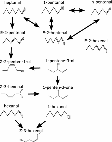
Constructed Bayesian network for 13 plant-derived compounds for beef, round and cherry tomatoes
Concluding remarks
Constructing graphically intuitive models has become a popular technique in metabolomics experiments (Morgenthal et al. 2006; Beal et al. 2005). Models like this allow us to understand the underlying biological processes involved in metabolic networks and reconstruct pathways. This knowledge is normally visualized by means of a directed graph, where the nodes of the graph correspond to variables and arrows in the graph are used to express statistical dependence and independence information.
The approach described in the present study proved useful to discover causal biochemical relationships in complex metabolomics data. The results are confirmed by previous observations on the same data as well as information found in literature. Methods such as Bayesian networks which are used for causal modeling of high-dimensional data are powerful tools in modeling of complex systems, since these approaches do take into account correlation methods before constructing an equivalent or exact causal relationship. Here we show how a Bayesian network can be used to analyze metabolomics data which is a powerful technique and helps us to get indepth understanding of the biological process. This method can be exploited further by coupling it with pathway databases in order to get exact and more plausible information to understand the process changes at hand. As more and more data become available these methods can outperform classical statistical techniques and be used to find novel biochemical pathways. We have shown here how this approach can be used for exploratory data analysis in searching for causal relationships in metabolomics. The resulting hypothesis can then be used to form the basis of subsequent analysis which can learn from data, take prior inputs from molecular biologist and update probabilities in the light of “new information” and/or “data”.
Electronic supplementary material
Below is the link to the electronic supplementary material.
Acknowledgments
The authors like to thank Centre for BioSystems Genomics (CBSG; http://www.cbsg.nl) for making the data available. This study was supported by grants from Biorange (http://www.nbic.nl) and Nutrigenomics Consortium (NGC; http://www.nutrigenomicsconsortium.nl).
Open Access
This article is distributed under the terms of the Creative Commons Attribution Noncommercial License which permits any noncommercial use, distribution, and reproduction in any medium, provided the original author(s) and source are credited.
References
- Baldwin E, Scott J, Shewmaker C, Schuch W. Flavor trivia and tomato aroma: Biochemistry and possible mechanisms for control of important aroma components. Hort Science. 2000;35:1013–1022. [Google Scholar]
- Beal MJ, Falciani F, Ghahramani Z, Rangel C, Wild DL. A Bayesian approach to reconstructing genetic regulatory networks with hidden factors. Bioinformatics. 2005;21(3):349–356. doi: 10.1093/bioinformatics/bti014. [DOI] [PubMed] [Google Scholar]
- Dellaert, F. (2002). The expectation maximization algorithm. Tech. rep., College of Computing, Georgia Institute of Technology.
- Eiceman, G., & Karpas, Z. (2005). Ion mobility spectrometry. USA: CRC Press.
- Elidan, G., & Friedman, N. (2003). The information bottleneck EM algorithm. In proceedings of UAI, Morgan Kaufmann (pp. 200–208).
- Fiehn, O., Kopka, J., Dormann, P., Altmann, T., Trethewey, R. N., & Willmitzer, L. (2000). Metabolite profiling for plant functional genomics. Nature Biotechnology, 18(11), 1157–1161. doi:org/10.1038/81137. [DOI] [PubMed]
- Friedman N, Linial M, Nachman I, Pe’er D. Using Bayesian networks to analyze expression data. J Comput Biol. 2000;7(3-4):601–620. doi: 10.1089/106652700750050961. [DOI] [PubMed] [Google Scholar]
- Gohlke R. Time-of-flight mass spectrometry and gas-liquid partition chromatography. Anal. Chem. 1959;31:535–41. doi: 10.1021/ac50164a024. [DOI] [Google Scholar]
- Heckerman, D. (1995). A tutorial on learning with Bayesian networks. Tech. rep., Microsoft Research.
- Husmeier, D., Dybowski, R., & Roberts, S. (2005). Probabilistic modeling in bioinformatics and medical informatics, (p. 504). New York: Springer.
- Jordan MI. Graphical models. Statistical Science. 2004;19:140–155. doi: 10.1214/088342304000000026. [DOI] [Google Scholar]
- Kalisch M, Buhlmann P. Estimating high-dimentional directed acyclic graphs with the PC-algorithm. Journal of Machine Learning Research. 2007;8:613–636. [Google Scholar]
- Kopka J, Fernie A, Weckwerth W, Gibon Y, Stitt M. Metabolite profiling in plant biology: Platforms and destinations. Genome Biol. 2004;5(6):109. doi: 10.1186/gb-2004-5-6-109. [DOI] [PMC free article] [PubMed] [Google Scholar]
- Meek C. Causal inference and causal explanation with background knowledge. Uncertainty in Artificial Intelligence. 1995;11:403–410. [Google Scholar]
- Moco S, Bino RJ, Vorst O. A liquid chromatography-mass spectrometry-based metabolome database for tomato. Plant Physiology. 2006;141(4):1205–1218. doi: 10.1104/pp.106.078428. [DOI] [PMC free article] [PubMed] [Google Scholar]
- Morgenthal K, Weckwerth W, Steuer R. Metabolomic networks in plants: Transitions from pattern recognition to biological interpretation. Biosystems. 2006;83(2-3):108–117. doi: 10.1016/j.biosystems.2005.05.017. [DOI] [PubMed] [Google Scholar]
- Murphy, K. P. (2002). Dynamic Bayesian networks. http://www.cs.ubc.ca/∼murphyk/Papers/dbnchapter.pdf.
- Opgen-Rhein R, Strimmer K. From correlation to causation networks: A simple approximate learning algorithm and its application to high-dimensional plant gene expression data. BMC Systems Biology. 2007;1:37. doi: 10.1186/1752-0509-1-37. [DOI] [PMC free article] [PubMed] [Google Scholar]
- Pearl, J. (1998). Probabilistic reasoning in intelligent systems: Networks of plausible inference. Menlo Park: Morgan Kaufmann.
- R Development Core Team. (2008). R: A language and environment for statistical computing. Vienna: Austria, ISBN 3-900051-07-0.
- Schauer N, Semel Y, Roessner U. Comprehensive metabolic profiling and phenotyping of interspecific introgression lines for tomato improvement. Nature Biotechnology. 2006;24(4):447–454. doi: 10.1038/nbt1192. [DOI] [PubMed] [Google Scholar]
- Sprites, P., Glymour, C., & Scheines, R. (2000). Causation, prediction and search. Cambridge: The MIT Press.
- Suizdak G. The expanding role of mass spectrometry in biotechnology. San Diego, CA: MCC Press; 2003. [Google Scholar]
- Tikunov Y, Lommen A, de Vos CHR, Verhoeven HA, Bino RJ, Hall RD, Bovy AG. A novel approach for nontargeted data analysis for metabolomics. Large-scale profiling of tomato fruit volatiles. Plant Physiology. 2005;139(3):1125–1137. doi: 10.1104/pp.105.068130. [DOI] [PMC free article] [PubMed] [Google Scholar]
- Tsamardinos I, Brown LE, Aliferis. CF. The max-min hill-climbing Bayesian network structure learning algorithm. Machine Learning. 2006;65:31–78. doi: 10.1007/s10994-006-6889-7. [DOI] [Google Scholar]
- Ursem R, Tikunov Y, Bovy A, van Berloo R, van Eeuwijk F. A correlation network approach to metabolic data analysis for tomato fruits. Euphytica. 2008;161:181–193. doi: 10.1007/s10681-008-9672-y. [DOI] [Google Scholar]
- Weckwerth W. Metabolomics in systems biology. Annual Review of Plant Biology. 2003;54:669–689. doi: 10.1146/annurev.arplant.54.031902.135014. [DOI] [PubMed] [Google Scholar]
- Yilmaz E. Oxylipin pathway in the biosynthesis of fresh tomato volatiles. Turk Biyoloji Dergisi. 2001;25:351–360. [Google Scholar]
- Yilmaz E, Tandon KS, Scott JW, Baldwin EA, Shewfelt RL. Absence of a clear relationship between lipid pathway enzymes and volatile compounds in fresh tomatoes. Plant Physiology. 2001;158:1111–1116. doi: 10.1078/0176-1617-00482. [DOI] [Google Scholar]
- Zou M, Conzen SD. A new dynamic Bayesian network (dbn) approach for identifying gene regulatory networks from time course microarray data. Bioinformatics. 2005;21(1):71–79. doi: 10.1093/bioinformatics/bth463. [DOI] [PubMed] [Google Scholar]
Associated Data
This section collects any data citations, data availability statements, or supplementary materials included in this article.


