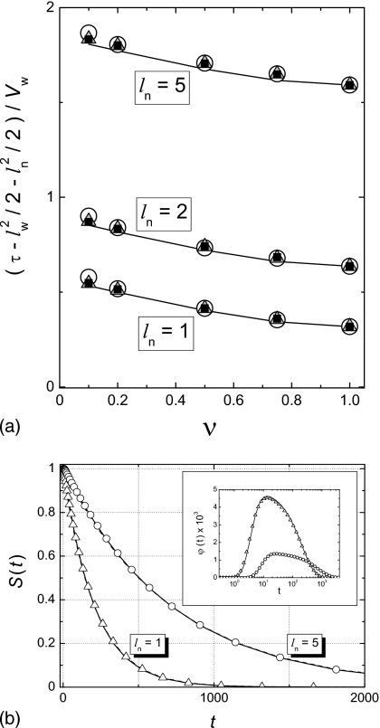
Figure 3.

Numerical test of the theory. We take a=D=1, i.e., we use a and a²∕D as units of length and time. As a consequence, ν=1∕b. In panel (a), solid curves show the ν-dependence of function $\left({\tau }_{\text{BH}}-l_w^2∕2-l_n^2∕2\right)∕V_w$, which is given by l_n∕π+1∕[4f(ν)] independently of l_w, Eq. 4.1. The curves represent the function at l_n=5,2,1 (from top to bottom). As ν→1,f(ν)→∞, and $\left({\tau }_{\text{BH}}-l_w^2∕2-l_n^2∕2\right)∕V_w$ approaches $\left({\tau }_{\text{F-J}}-l_w^2∕2-l_n^2∕2\right)∕V_w$, which is equal to l_n∕π for all ν, 0<ν<1, Eq. 4.2. Symbols are numerical results for $\left(\tau -l_w^2∕2-l_n^2∕2\right)∕V_w$ at the same l_n and l_w=2 (circles), l_w=5 (triangles), and l_w=10 (squares). In panel (b), solid curves are the survival probabilities S(t) and the lifetime probability densities ϕ(t) (inset) obtained by numerically inverting the Laplace transforms $\widehat{S}\left(s\right)$ and $\widehat{\varphi }\left(s\right)$ given in Eqs. 2.18, 2.17 at l_w=b=5 and l_n=1,5 (D_w=D_n=1). Symbols are numerical results: triangles for l_n=1 and circles for l_n=5.