Simultaneous navigation of multiple Pareto surfaces, with an application to multicriteria IMRT planning with multiple beam angle configurations

Abstract

Purpose: To introduce a method to simultaneously explore a collection of Pareto surfaces. The method will allow radiotherapy treatment planners to interactively explore treatment plans for different beam angle configurations as well as different treatment modalities.

Methods: The authors assume a convex optimization setting and represent the Pareto surface for each modality or given beam set by a set of discrete points on the surface. Weighted averages of these discrete points produce a continuous representation of each Pareto surface. The authors calculate a set of Pareto surfaces and use linear programming to navigate across the individual surfaces, allowing switches between surfaces. The switches are organized such that the plan profits in the requested way, while trying to keep the change in dose as small as possible.

Results: The system is demonstrated on a phantom pancreas IMRT case using 100 different five beam configurations and a multicriteria formulation with six objectives. The system has intuitive behavior and is easy to control. Also, because the underlying linear programs are small, the system is fast enough to offer real-time exploration for the Pareto surfaces of the given beam configurations.

Conclusions: The system presented offers a sound starting point for building clinical systems for multicriteria exploration of different modalities and offers a controllable way to explore hundreds of beam angle configurations in IMRT planning, allowing the users to focus their attention on the dose distribution and treatment planning objectives instead of spending excessive time on the technicalities of delivery.

INTRODUCTION

In radiation therapy, multicriteria optimization with real-time navigation of Pareto surfaces (PSs) is emerging as a fast and informative strategy for intensity modulated radiation therapy (IMRT) treatment planning.¹ In this context, the Pareto surface is represented by a set of treatment plans and their linear combinations (i.e., the linear combinations of the fluence vectors), each plan having varying strengths and weaknesses regarding the treatment planning objectives. During the navigation session, the user interface allows the planner to move along the high dimensional Pareto surface (in radiation therapy, there are typically somewhere between five and ten different objectives being traded off) by adjusting sliders, one for each of the underlying objectives. This approach is theoretically justified when the underlying optimization problem is convex, since then the Pareto surface is convex and linear combinations of Pareto optimal plans are feasible.^{2, 3}

In IMRT radiation treatment planning, when one includes the beam angles as decision variables, the optimization problem is no longer convex (e.g., Refs. ^{4, 5}). One way to understand why the IMRT problem with beam angle optimization (BAO) is nonconvex is to see that given two different “good” angle sets, there is no guarantee that the angle set midway between these two angles sets is good or even feasible for that matter. For instance, angle set 1 may avoid a certain critical structure and angle set 2 might avoid it in a different way, but the angle set created by averaging the angle locations could have an angle pass right through that critical structure. Because of this nonconvexity, determining the Pareto surface to an IMRT problem where beam angles are included as optimization variables is a problem of global nonconvex optimization, where no solution method has yet been demonstrated. A practical alternative to attempting to determine and navigate a single BAO Pareto surface, where the beam angle configuration would vary continuously across the surface, is to compute Pareto surfaces for a large set of beam configurations and provide a method to navigate the collection of surfaces.

Multiple Pareto surfaces might arise in other contexts within radiotherapy planning, for example, users might compute different Pareto surfaces for various delivery modalities (protons, IMRT, and arc delivery). The methods presented here can be used for the interactive exploration of sets of those surfaces as well. In this paper, however, we use the beam angle problem for the source of multiple Pareto surfaces. We introduce a new method of navigating on a single Pareto surface, and then extend this method to the navigation of a collection of Pareto surfaces.

METHODS

We consider a collection of Pareto surfaces. Each Pareto surface has the same underlying set of convex objective functions and the feasible space for the multiobjective formulation is convex. In the navigation process we are solely working with the precomputed plans and linear combinations of these plans. Therefore, for the navigation we use the term “Pareto surface” to mean undominated convex combinations of the precomputed plans (for example, the piecewise linear curve shown in Fig. 1). While strictly speaking this is just an approximation of the Pareto surface, we assume there are a sufficient number of well-distributed Pareto optimal points calculated so that this is a close approximation. Relevant methods to compute well-distributed points on a Pareto surface are given in Refs. ^{6, 7, 8}.

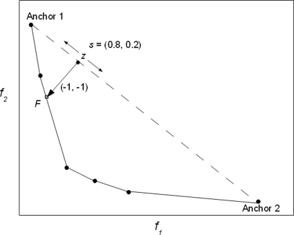
Figure 1.

A depiction of the navigation of a single Pareto surface using the piercing algorithm. User navigation alters the point z on the dashed line connecting the two anchor points by altering the convex combination s of the anchor points that defines that point. The Pareto surface point F that is associated with that point z is the point indicated by the small square and is found by moving from z in the direction of (−1,−1,…).

We represent each Pareto surface as a matrix, with rows corresponding to the Pareto optimal plans and the columns corresponding to the objectives. Let P_i be the matrix representing the ith Pareto surface. Thus, P_i is an m×n matrix, where m is the number of points on the surface and n is the number of objectives. Note that each of our surfaces could have a different number of points, but in this paper we will assume for simplicity that each surface is made up of same number of points m. We assume that m>n.

Navigating the surface of a single Pareto surface

Here we present a new method for the navigation of a single PS which naturally extends to the navigation of multiple surfaces. We assume that the first n points on the PS are the anchor plans (i.e., the best you can do in each objective individually).

Each of the n anchor plans (“plans” and “points” used interchangeably throughout) is a point in the n dimensional Pareto space and we associate these plans with the objectives that they minimize. The user navigates across the PS by increasing or decreasing the significance of each of the anchor plans in the following way.

Let s be a convex combination vector of length n. That is, the components of s are non-negative and sum to 1. A convex combination of the n anchor plans is not necessarily Pareto optimal, but a unique Pareto optimal point can be associated with the convex combination in the following way.

Let Q denote the first n rows of the PS matrix P. Let z=s^′Q be the convex combination location. Since our underlying optimization problem is convex, z is a feasible solution. Now we imagine a vector emanating from z and pointing in the direction (−1,−1,…). The problem of finding the point along the Pareto surface along this direction can be solved by a small linear program.^{1, 9} The formulation is as follows:

$$\text{min}h,$$ (1)

$$s.t.h\ge y_i-z_i,\text{for}i=\mathrm{1..}n,$$

$$y=F+q,$$

$$F=v^{\prime }P,$$

$$\sum v_i=1,$$

$$v,q\ge 0.$$

Here F is a point on the Pareto surface. A slack variable q is included for the case when the line from z in the direction (−1,−1,…) does not intersect the surface. In that case q is nonzero (otherwise, y=F as in Fig. 1). We call this the piercing step since it is visualized as piercing the PS. This formulation, called a scalarization method, is proved in Ref. 9 to always be feasible and always yield a Pareto optimal point (again, in our case subject to the error stemming from our discrete approximation of the PS).

What remains is to map the user request, increasing or decreasing the relative contribution of each objective, into changing the vector s. This is handled in the following way.

We present two arrow buttons for each objective, one up and one down, as well as a lock button. Consider the user clicking the up button for objective j. Clicking the up arrow for j means increase the contribution of that anchor plan, so we should increase s_j. Let inc be the amount by which s_j is changed. For any plan that is locked, we do not change the s for that plan. Let SNF be equal to the sum of the not fixed s_i, not including the one we are changing, s_j. SNF is the wiggle room we have to work with. With inc=0.1 (i.e., a 10% step size in navigation), we consider two cases:

• Case 1: SNF>0.1 (and therefore s_j<0.9). This is our “normal” situation where we have some wiggle room, so we take a full step of size inc=0.1 (i.e., s_j new=s_j+inc).

• Case 2: SNF<0.1. Here we have less than 0.1 of wiggle room, so we take a smaller step. Specifically, we take inc=1∕3 SNF.

Now, we update the other s values, the ones that are not locked, in proportion to their size. This works out algebraically as s_i new=g⋅s_i, where g=1−inc∕SNF. A downward click is antisymmetric to the upward click so details are omitted. Also note that inc=0.1 and inc=SNF∕3 are arbitrary and could be chosen differently for larger or smaller navigation steps.

With these details in place, the entire process of on-surface navigation of a single PS can be summarized: When the user clicks the up or down arrow for a particular objective, the convex combination vector s is updated according to case 1 or 2 above, and then the piercing linear program (1) is solved to push the solution to the PS, at which point the dose distribution and other visualizations of the current solution are updated.

Navigating multiple Pareto surfaces

Implementing a navigation on multiple Pareto surfaces needs a method for switching between surfaces. The system we present has a switch request coupled with one of the objectives. A switch should move to a surface which offers an improvement in that objective, and should also meet the following two requirements. First, the new plan found after the switch should be Pareto optimal. Second, the dose distribution should not change too much. We ensure the former by optimizing the position on the new surface. The latter needs the following preprocessing, to make sure a “close” surface is selected.

For each surface and each objective, we store the closest PS that offers an improvement in the particular objective. In the base of beam angle sets as the underlying source of the multiple Pareto surfaces, it is natural to define closeness in terms of the “distance” between the beam angle configurations of the corresponding Pareto surfaces. This way, as the user is navigating and switching surfaces, the process is as smooth as possible.

We assume each angle configuration has the same number of angles. We pair the beam angles of two sets such that the sum of the distances is as small as possible using a matching problem and define this to be the distance of two given beam angle sets. Determining the optimal pairing which minimizes the sum of the angle differences can efficiently be solved by linear programming (e.g., Ref. 10).

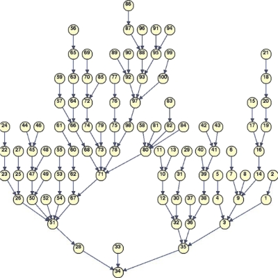
With the distances between all angles sets computed, we do the following for each angle set. For each objective, we find the closest angle set that offers an improvement in the objective (a beam angle set offers an improvement in an objective if its anchor point solution for that objective is lower), and assign that as the neighboring angle set. Figure 2 shows the results for objective function 2 for the case presented in Sec. 2C. The results are shown as a tree structure with each beam angle configuration shown as a node pointing to the next closest improving beam angle set node.

Figure 2.

Tree structure of 100 beam angle configurations showing nearest neighbors for each beam angle set regarding improving objective function 2, mean kidney 1 dose. Angle set 34 is the absolute best for this objective function. For all other nodes, for example, the uppermost node representing angle set 86, the node points down to the closest angle set that offers an improvement in objective 2.

The system offers two styles regarding surface switching: Manual and automatic. In manual switching, navigation moves do not result in surface changes. This is helpful when the user wants more control: A surface switch can result in a sudden jump in dose distribution characteristics. In automatic switching, after the user clicks to improve or worsen any objective, the piercing optimization [Eq. 1] is run for all of the Pareto surfaces and the surface with the smallest optimal value h^∗ is chosen as the next surface, it being the dominating solution.

In both the automatic and manual switching, the user can request a surface change at any time. This is done when the user desires to move to the next best surface for a particular objective. This is handled as follows.

First, the place on the new surface (the surface given by the information shown in Fig. 2) to move to is found which best matches the current objective vector. This is found by solving the following linear program. Let G be the current location on the current PS. Let P_N be the next Pareto surface to move to, and let (P_N)ⁱ be the ith column of the P_N matrix, v is the convex combination vector to be solved for.

$$\text{min}y,$$ (2)

$$s.t.\text{y}\ge \left|G_i-v^{\prime }{\left(P_N\right)}^i\right|,\text{for}\text{all}i,$$

$$v\ge 0,$$

$$\sum v_i=1.$$

Notice that any deviation between G and the new point v^′ (P_N), is minimized by pushing the decision variable y down. After solving this we have a new point in objective function space. Navigation control happens in the space of the convex hull of the anchor plans though. Therefore, we solve the following linear set of equations to map the location found in the above optimization back onto the anchor points’ plane. Let q be the new point q=v^∗′P_N. Let Q denote the first n rows of P_N. We want to solve for the amount we move in the (1,1,1,…) direction from the point q until we are on the hyperplane which passes through the anchor plans (the rows of Q). That is, we want to solve for the scalar quantity t such that q⁺t^∗(1,1,1,…)=s^∗Q. This is n equations with n+1 unknowns, the s vector plus the scalar t. The convex combination constraint on s gives us one more equation so we can solve for all the quantities. Notice this allows for negative values which sometimes arise if the Pareto surface is skewed, such that the outward projection of the point q does not intersect the convex hull of the anchor plans (this cannot happen in 2D). Negative values are simply set to 0 and the resulting s vector (i.e., the first n components of x) is renormalized. At this point, if there are active locks, then the locked values of the convex combination s are reset to their locked values and the other values are scaled such that the s vector sums to 1 again. Another option is to remove the locks during a surface switch since a surface switch might dramatically change where you are in objective space, and in that scenario, the locks have less significance. Either way, once s is set, the piercing algorithm [Eq. 1] is performed to ensure the new plan being displayed is on the PS.

Choosing the set of beam angle configurations

We use the following approach for obtaining a set of Pareto surfaces in the beam angle context. Note this subsection is not needed to understand the main algorithms of this paper, but is included for completeness.

In choosing a finite set of beam angle configurations we balance between (1) having the angles configurations such that each has a close neighbor so that there is some smoothness to the navigation when the active surface changes and (2) widely spanning the space of angle configurations. We have chosen the following approach to balance these two goals.

We choose an angular spacing grid of Δ=5°. The first angle configuration in our set is an equispaced angle set (rounded to the 5° degree grid). From there, we generate the next set by, for each beam, randomly choosing to increase or decrease the angle by Δ, or keep it the same, each with equal likelihood. If this new angle configuration has not been found yet and does not violate a “beams too close” rule (we use 15° as our cutoff), it is added to the set. The random search proceeds then from that new set, and goes until we have the desired number of beam angle configurations. Instead of this linear advancing random walk to populate the beam angle configuration space, one could also branch at each step with two or more branches, creating more of a tree structure. This would tend to cover less of the beam angle space, but the surface switching would be generally smoother.

DEMONSTRATION OF SYSTEM

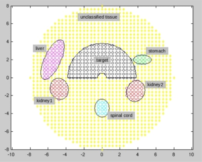
We use a 2D phantom representing a pancreas case. Pancreas cases are good studies for beam angle optimization because many critical structures are located around the target.¹¹ Figure 3 shows the patient geometry used in this study. We use five angles in each angle set, and a total of 100 angle sets. The multicriteria optimization problem has six objectives, all minimizations: (1) Mean liver dose, (2) mean kidney 1 dose, (3) mean kidney 2 dose, (4) upper ramp at 25 Gy for the stomach, (5) upper ramp at 25 Gy for the unclassified tissue, and (6) lower ramp at Rx=50.4 Gy for the target. Ramp functions linearly penalize any voxel above or below the ramp level, by an amount equal to the distance to the ramp point.¹²

Figure 3.

Patient geometry (2D) used for demonstrating the multiple Pareto surface navigation system. Target and organs at risk are shown. Spinal cord is not used as an objective in this model because in clinical pancreas cases, cord is not close enough to the target to consider it an organ at risk. Scale of axes is centimeters and individual voxels are shown, each is 0.4×0.4 cm². Beamlet size is 1 cm.

Hard constraints for the formulation are: 0.95^∗Rx≤target voxel dose≤1.12^∗Rx and all doses≤1.12^∗Rx. For each angle configuration we compute a Pareto surface of exactly seven plans, the anchor plans, and then a single equiweighted plan. Voxel size is 0.4×0.4 cm² and beamlet size is 1 cm. The dose calculation used is the triple Gaussian pencil beam model from Ref. 13. Note that any convex functions, such as equivalent uniform dose or quadratic deviation functions, can also be used in this framework.

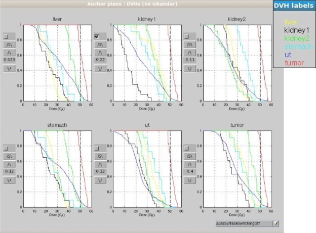
Figure 4 displays the main navigation dashboard. In this version of the dashboard, each of the underlying six objectives is represented by its dose volume histogram. Controls are discussed in the figure caption.

Figure 4.

Navigation dashboard for multiple Pareto surface navigation. Six anchor plans with their dose volume histograms (DVHs) are shown. For each plan, four control buttons appear at the left of the DVH. The increase arrow ∧ is used to increase the contribution of this type of plan, and the downward facing arrow ∨ is for the opposite. The buttons labeled S caused the active surface that is being navigated to switch to the closest other surface in the computed set, which offers the chance for more improvement regarding that objective. The check box is used as a constraint. If this is clicked, as it is for kidney 1, then the contribution of the kidney 1 plan is fixed at the value shown, in this case 0.22. The values shown in the text boxes for each plan constitute the s vector in the text.

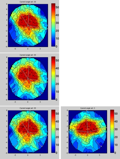
Figure 5 shows a sequence of navigation steps, two steps improving the kidney 2 objective and the third step where the surface is changed to the closest surface that has better plans regarding kidney 2 than the original surface.

Figure 5.

A sequence of four navigation steps for improving kidney 2, the structure at the lower right of the target. From the top downward are steps on the same Pareto surface. Then, for the final step, a few manual surface changes were requested, and the system moved to surface of angle set 3, which shows a better beam configuration for avoiding kidney 2. In the demonstration system, DVH plots are updated as well with every navigation move (not shown).

DISCUSSION AND CONCLUSIONS

This paper introduces, to the authors’ knowledge, the first report on navigating multiple Pareto surfaces, and the first use of the piercing scalarization method using a navigation reference point lying on the hyperplane through the n anchor plans (for a single Pareto surface, this is the main difference between the current method and the method presented in Ref. 1). The lower envelope of the collection of Pareto surfaces is the entity over which we would like to navigate. Rather than explicitly calculating this lower envelope, our method navigates it implicitly, and by doing so avoids the difficult mathematical task of representing the boundaries where the Pareto patches join. Furthermore, the lower envelope of patched Pareto surfaces is in general nonconvex and there is no guarantee that it is even connected (i.e., there could be holes). Finally, by storing all of the surfaces in entirety, our system allows users to explore each surface in its entirety. Forcing the users to only be able to view plans that are globally Pareto optimal (i.e., only the lower envelope) results in more restrictive and less smooth navigation.

The benefits of the piercing method, in addition to its simplicity, are: (1) It is an easy way to stay on Pareto surface and (2) it easily extends to multiple Pareto surfaces. The drawback of the method as presented is that the user control is on the hyperplane connecting the anchor plans instead of directly on the objective function values. However, this is largely alleviated by the fact that objective function values can be displayed in real-time during the navigation, and objective value constraints can be invoked during the navigation process (e.g., Ref. 1).

We have demonstrated the navigation of multiple Pareto surfaces by using multiple beam angle configurations for IMRT, and switching to a close surface is straightforward in this context because it is easy to define the closeness of Pareto surfaces by the closeness of the underlying beam angle sets. If multiple Pareto surface navigation is used for comparing different modalities (protons versus photons, for example), it is left to decide if automatic surface switching would be implemented, and how to select the next “closest” surface to move to.

References

- Monz M., Küfer K. -H., Bortfeld T., and Thieke C., “Pareto navigation—Algorithmic foundation of interactive multi-criteria IMRT planning,” Phys. Med. Biol. 53(4), 985–998 (2008). 10.1088/0031-9155/53/4/011 [DOI] [PubMed] [Google Scholar]
- Romeijn H. E., Dempsey J., and Li J., “A unifying framework for multi-criteria fluence map optimization models,” Phys. Med. Biol. 49(10), 1991–2013 (2004). 10.1088/0031-9155/49/10/011 [DOI] [PubMed] [Google Scholar]
- Jin Y. and Sendhoff B., “Constructing dynamic optimization test problems using the multi-objective optimization concept,” Applications of Evolutionary Computing, Lecture Notes in Computer Science Vol. 3005, edited by Raidl G.et al. (Springer, Berlin∕Heidelberg, 2004), pp. 525–536. [Google Scholar]
- Lim G., Choi J., and Mohan R., “Iterative solution methods for beam angle and fluence map optimization in intensity modulated radiation therapy planning,” OR-Spectrum 30(2), 289–309 (2008). 10.1007/s00291-007-0096-1 [DOI] [Google Scholar]
- Pugachev A. B., Boyer A., and Xing L., “Beam orientation optimization in intensity-modulated radiation treatment planning,” Med. Phys. 27(6), 1238–1245 (2000). 10.1118/1.599001 [DOI] [PubMed] [Google Scholar]
- Craft D. L., Halabi T., Shih H., and Bortfeld T., “Approximating convex Pareto surfaces in multiobjective radiotherapy planning,” Med. Phys. 33(9), 3399–3407 (2006). 10.1118/1.2335486 [DOI] [PubMed] [Google Scholar]
- Messac A. and Mattson C., “Normal constraint method with guarantee of even representation of complete Pareto frontier,” Proceedings of the 45th AIAA‘ASME‘ASCE‘AHS‘ASC Structures, Structural Dynamics, and Materials Conference, 2004, Vol. 42, Issue 10, pp. 2101–2111 (unpublished).
- Serna J. I., Monz M., Küfer K. -H., and Thieke C., “Trade-off bounds for Pareto surface approximation in multi-criteria IMRT planning,” Phys. Med. Biol. 54(20), 6299–6311 (2009). 10.1088/0031-9155/54/20/018 [DOI] [PubMed] [Google Scholar]
- Pascoletti A. and Serafmi P., “Scalarizing vector optimization problems,” J. Optim. Theory Appl. 42(4), 499–524 (1984). 10.1007/BF00934564 [DOI] [Google Scholar]
- Bertsimas D. and Tsitsiklis J., Introduction to Linear Optimization (Athena Scientific, Nashua, 1997). [Google Scholar]
- Woudstra E., Heijmen B., and Storchi P., “A comparison of an algorithm for automated sequential beam orientation selection (Cycle) with simulated annealing,” Phys. Med. Biol. 53(8), 2003–2018 (2008). 10.1088/0031-9155/53/8/001 [DOI] [PubMed] [Google Scholar]
- Craft D. and Bortfeld T., “How many plans are needed in an IMRT multi-objective plan database?,” Phys. Med. Biol. 53(11), 2785–2796 (2008). 10.1088/0031-9155/53/11/002 [DOI] [PubMed] [Google Scholar]
- Ulmer W. and Harder D., “A triple Gaussian pencil beam model for photon beam treatment planning,” Z. Med. Phys. 5(1), 25–30 (1995). [Google Scholar]