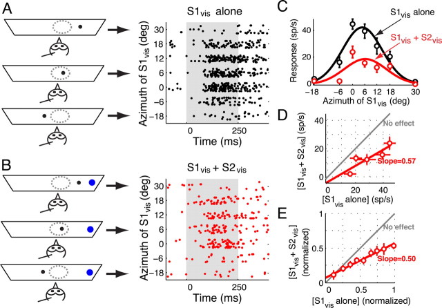
Figure 3.
Effect of a distant visual competitor on visual tuning curves. A, Left, Schematic representation of the experimental setup showing a single looming stimulus (black dot) at various locations. The arrows point to the responses obtained at each of the depicted stimulus configurations. Right, Raster display of neuronal responses to a single looming stimulus (S1vis) presented at various azimuthal locations. Stimulus duration = 250 ms. Positive (negative) azimuthal values represent contralateral (ipsilateral) locations relative to the recording site. B, Left, Schematic representation of stimulus locations when two looming visual stimuli were presented. One stimulus (competitor, S2vis, shown as a blue dot) was always far outside the RF (30° lateral) while another (S1vis, shown as a black dot) traversed the RF in azimuth. Right, Raster display of the neuronal responses when both S1vis and S2vis were presented. Conventions as in A. C, Responses of the OTi-d site plotted as a function of the azimuth of the S1vis stimulus when it was presented alone (black) or together with the S2vis competitor (red). The data indicate mean ± SEM. The azimuthal tuning curves, obtained as the best-fit Gaussian to the responses in each condition, are also shown. D, Responses to the S1vis and S2vis stimuli presented together compared with the responses to the S1vis stimulus alone. Responses to only those locations at which S1vis was inside the RF (i.e., locations at which S1vis elicited above-baseline activity; see Materials and Methods) are plotted. Linear regression of these responses yielded a fit with a slope of 0.57 that was significantly different from 1 (p < 0.05, Materials and Methods) and an intercept of −3.6 spikes/s that was not significantly different from 0 (p = 0.6). The gray line indicates no effect of the competitor stimulus. E, Population summary (n = 25 sites, 113 points). All responses at each site were normalized to the maximum response obtained at that site when S1vis was presented alone. Data from all the sites were binned based on the values of the normalized responses to S1vis alone (bin size 0.15) and plotted (mean ± SEM). Linear regression of these normalized and binned responses yielded a fit with a slope (1/divisive factor) of 0.50 (significantly different from 1, p < 0.05; see Materials and Methods), and a y-intercept (additive factor) of 7% (significantly different from 0, p = 0.02; see Materials and Methods).

