Figure 7.
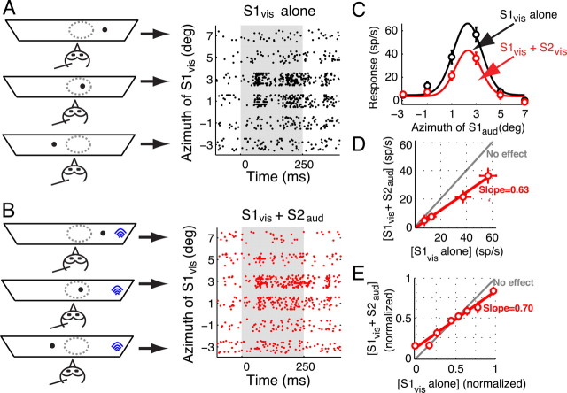
Effect of a distant auditory competitor on visual tuning curves. A, Left, Schematic representation of the experimental set-up showing a single looming stimulus (black dot) at various locations. The arrows point to the responses obtained with each of the depicted stimulus configurations. Right, Raster display of neuronal responses to a single looming stimulus (S1vis) presented at various azimuthal locations. Stimulus duration = 250 ms. Positive (negative) azimuthal values represent contralateral (ipsilateral) locations relative to the recording site. B, Left, Schematic representation of stimulus locations when visual and auditory stimuli were simultaneously presented. The auditory stimulus (competitor, S2aud, shown as blue arcs) was always far outside the auditory RF (30° lateral) while the visual stimulus (S1vis, shown as a black dot) traversed the visual RF in azimuth. Right, Raster display of the neuronal responses when both S1vis and S2aud were presented. Conventions as in A. C, Responses of an OTi-d site plotted as a function of the azimuth of a looming visual stimulus (S1vis) presented alone (black), or together with a noise burst, auditory competitor (S2aud; red). The auditory stimulus was located 30° lateral to the RF center. The properties of the stimuli are given in the text. The data indicate mean ± SEM. The azimuthal tuning curves, obtained as the best-fit Gaussian to the responses in each condition, are also shown. D, Responses to the S1vis and S2aud stimuli presented together compared with the responses to the S1vis stimulus alone. Linear regression yielded a fit with a slope of 0.63 (significantly different from 1, p < 0.05; Materials and Methods) and an intercept that was not significantly different from 0. The gray line indicates no effect of the competitor stimulus. E, Population summary (n = 14 sites, 64 points). Responses to S1vis presented along with S2aud and responses to S1vis alone are normalized, binned and plotted as described for Figure 3E. Linear regression of these normalized and binned responses yielded a fit with a slope (1/divisive factor) of 0.70 (significantly different from 1, p < 0.05; Materials and Methods), and a y-intercept (additive factor) of 13% in normalized coordinates (significantly different from 0, p = 0.005, see Materials and Methods).

