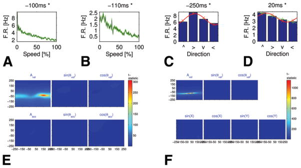
Fig. 2.

Tuning curves for speed and direction, and PCC in the SMA proper. A and B: Speed tuning curves showing a decreasing monotonic relationship between the firing rates (F.R., in Hz) and speed percentiles (Case 2). Each graph refers to a different unit (A: multiunit, B: single unit). The background (green) area around each curve represents the standard error. The leftmost point in each plot (marked 0) describes the firing rate during rest (speed = 0), whereas points 1–100 are the average firing rate during percentiles of in-motion speed. Both units had a significant monotonic relationship. Above each graph is its time lag in milliseconds (negative values indicate that firing precedes motion). The decrease in firing rate with motion speed is appreciable. C and D: Bar graphs showing selectivity to direction of motion in 2 single neurons (Case 6): firing rate versus the direction of movement (indicated as the up, right, down, and left arrows on the x axis). Because cosine tuning curves are very common, especially in M1 (see Georgopoulos et al.), we fit each graph with a cosine function (red line). In C, the cosine tuning curve fits well (R² = 0.91, MSRE = 0.06). In D, R² is relatively low for the cosine model (R² = 0.84, MSRE = 0.06); the linear model (green line) provides a better explanation for the data (R² = 0.985, MSRE = 0.02). E and F: Graphs showing the t-statistic of the PCCMs between firing rate and velocity independent of linear correlation with acceleration (in E) or position (in F) at multiple time lags. The PCCMs are as follows: upper rows, speed, sin(θ_v), and cos(θ_v); lower rows, magnitude of the acceleration vector, sin(θ_a), and cos(θ_a) in panel E and sin(kx), cos(kx), sin(ky), and cos(ky) in panel F (see Appendix 3 for an explanation of the position representation). Both panels E and F (upper left) show strong stripes for the matrices related to speed, which indicates a high correlation with speed that is independent of acceleration and position.