
Figure 4.
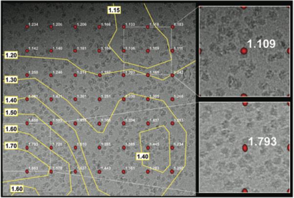
Example of a 40962 pixel CCD image at 50,000X and 45° tilt exhibiting BIM. This image would have been marked as bad in the manual evaluation even though only a small region in the lower left corner is clearly showing BIM. In this image the power spectrum peaks that were used in the computer evaluation are shown in red, centered over the 10242 pixel areas from which they were calculated. Next to each peak in white text is the computed score assigned to that region. The yellow contour lines were generated using Matlab, each encloses an image area with BIM greater than or equal to the shown score (found using interpolation). On the right, the lowest and highest scoring regions from the image are expanded for clearer visibility.