
Fig. 2.
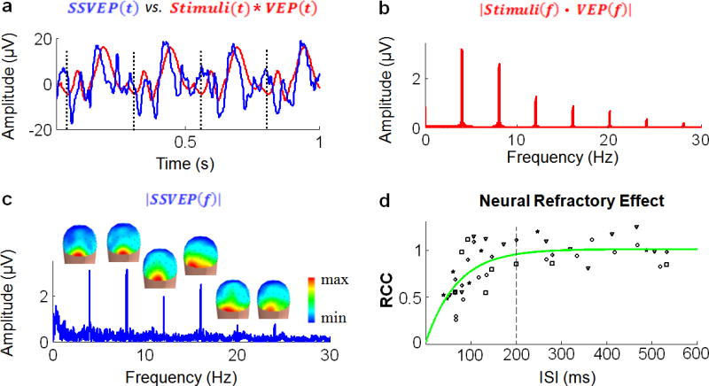
Neural response linearity/nonlinearity. a. Example of a 1-s period of the SSVEP signal measured from Oz is shown in blue. Corresponding linear prediction, derived by convolving the stimuli with the VEP signal at Oz, is shown in red. Vertical dashed lines represent the onsets of 4-Hz visual stimuli. b. Amplitude spectrum of the predicted SSVEP (red curve). c. Amplitude spectrum of the SSVEP measured from Oz (blue curve). Spatial distribution of the SSVEP amplitudes at the stimulus frequency (4 Hz) and its harmonic frequencies (8, 12, 16, 20, 24 Hz) are shown as 3-D scalp maps. d. Scatter-plot of the RCC values obtained from individual subjects at various ISIs (displayed as different symbols). An exponential function fitting the RCC-ISI values is illustrated by a curve in green. Vertical dashed line represents a neural refractory period of 200 ms. As such, neural response to repeated stimuli with ISI>200 ms is approximately linear (0.95<RCC≤1.01). When ISI<200 ms, the steady-state neural response is nonlinear (RCC<0.95). The shorter the ISI, the larger the degree of neural response nonlinearity.