
Fig. 3.
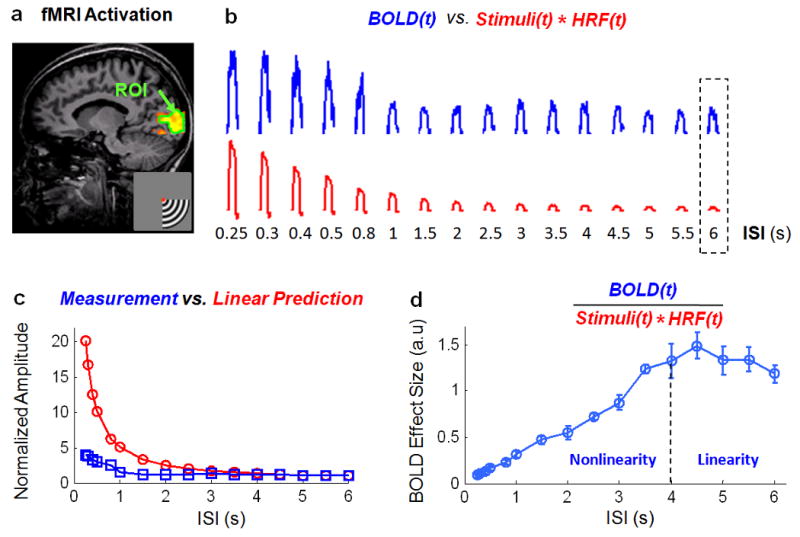
BOLD nonlinearity. a. ROI (surrounded by the green line) selected from the fMRI activation (red-to-yellow) within the upper calcarine sulcus, in response to stimuli presented in the lower-right quadrant of the visual field. b. Group-averaged (n=10) fMRI signals within the ROI shown in a, generated by a 30-s block of stimuli with ISIs from 0.25 to 6 s, are shown in blue. Corresponding regressors, derived by convolving the stimuli with the HRF, are shown in red. c. Steady-state heights of the measured fMRI signals (blue) and the corresponding regressors (red) are plotted as functions of the ISI, after normalizing (to 1) both the measured and modeled steady-state heights when ISI=6 s. d. Ratio between the measured fMRI signal and the regressor (i.e. the BOLD effect size) is plotted as a function of the ISI. Circles represent the group means. Error bars represent the standard errors of the mean (s.e.m) across subjects. The BOLD responses are approximately linear when ISI>4 s (marked by the vertical dashed line). When ISI<4 s, the BOLD responses are nonlinear. The shorter the ISI, the larger the degree of BOLD nonlinearity.