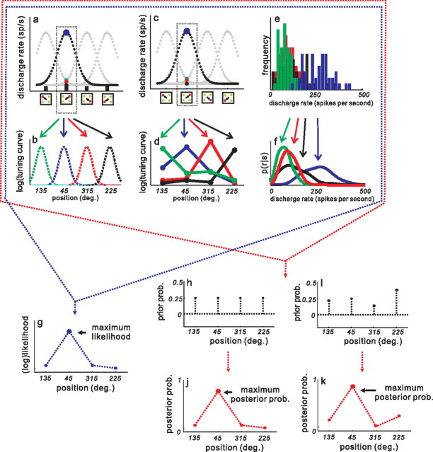
Figure 2.

Computing the posterior distribution across saccade choices. a, Simulated, idealized responses (in spikes per second) of four SC neurons in the four different target conditions of the task. Small squares on the abscissa show the four possible stimulus configurations of the task. The four curves simulate the activity of each neuron in each of the four possible conditions. For display, these data were simulated as Gaussian functions with σ = 40°. Each Gaussian peak was shifted by 90° to represent the four possible locations. Each simulated response shows a peak discharge when the target corresponds to the preferred location for the neuron and shows a reduced level of discharge as the target moves away from the preferred location. The dotted rectangle around the black simulated response shows an example response whose peak discharge (blue circle) appears for targets located at 45° and a reduced response for target locations elsewhere. The green dot, red dot, and black dot show the simulated discharge rate for the other three neurons when the target appears outside of their RF. b, Simulated weights for SC neurons. Each tuning curve represents the probability of neuronal discharge given a stimulus position from 0 to 359° (in steps of 0.1°). The tuning curves were simulated as Gaussian functions of equal amplitude (arbitrary units) and widths of 20.6° (Edelman and Keller, 1998). The logs of these Gaussian functions were used as weights. The green curve shows the weight for the neurons with the highest discharge rate in the 135° target condition. The blue curve shows the weight for the neurons with peak rates in the 45° target condition. The red and cyan curves show weights for the neurons with peak rates in the 315° and 225° target conditions, respectively. c, The same as in a. d, Each point is the measured discharge from an SC neuron when monkeys made saccades to one of each of the four possible locations. e, Frequency histogram of discharge rates measured from the sets of four neurons in the four possible target conditions across all datasets. The activity of target neurons is shown in the blue bars, whereas the activity of distractor neurons is shown in the green, red, and black bars. These histograms formed the basis for the density estimation (see Materials and Methods for details). f, The result of the density estimation (smooth histograms in e—see Materials and Methods) is the likelihood of a response given a particular saccade choice. Distractor neurons are green, red, and black. The target neurons are blue. g, Without incorporating a prior probability distribution the result is a (log) likelihood distribution. h, The uniform prior probability distribution. Each dot shows the probability of one saccade choice. Since the target could appear in each of the four locations with equal probability, the distribution is uniform. i, Same as in h but using a simulated, nonuniform prior distribution (see Materials and Methods). j, Estimated posterior probability distribution for one example target condition (45°). Multiplying all four conditional probability across the four neurons and the prior, results in the posterior probability for the example target condition across the four neurons. k, Same as in j for the distribution using a nonuniform prior.