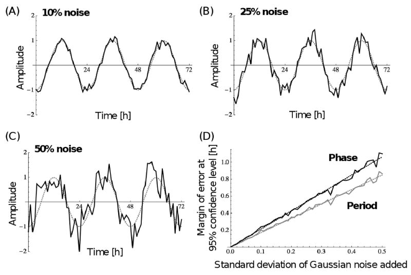
Fig. 2.

Robustness of the algorithm towards noise. (A) Example graph of an ideal sinusoidal curve with 24 h period and amplitude of 1 (dotted gray line), from which hourly points were sampled and random variables added to the amplitude (solid black line), whose mean is zero and whose standard deviation is 0.1 or 10%. (B) Same as in (A) except that the standard deviation of the random variables is 0.25 or 25%. (C) Same as in (A) except that the standard deviation of the random variables is 0.5 or 50%. (D) Margin of error at the 95% confidence level for the period (gray) and phase (black) for various standard deviations of the random variables. Data were derived from 250 random data sets per standard deviation. Standard deviations were evaluated at 0.01 intervals. Each dotted line represents the linear least-squares fit.