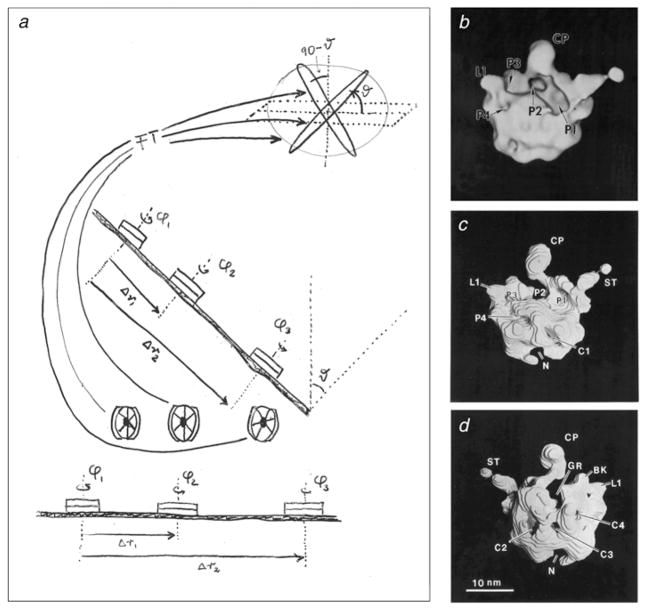
Fig. 5.

Random–conical reconstruction. (a) Principle of the random–conical data collection method. Two images are taken of the same field of molecules. Only molecules are considered that present the same view on the grid. Azimuthal angles are obtained by aligning the images of the untilted micrograph. Thus, with both azimuth and tilt angles known, the Fourier transform of each projection can be properly placed into the 3D Fourier reference frame of the molecule. From J. Frank (unpublished hand-drawing on overhead transparency, 1979). (b–d) Density map of the 50S ribosomal subunit from E. coli, the first 3D reconstruction using the random–conical data collection method. (a) Surface representation of intersubunit face; (b, c) higher-threshold solid model obtained by stacking of contoured slices, viewed from front and back. The subunit was negatively stained with uranyl acetate and air-dried, which accounts for the partial flattening. The ridge of the deep groove running horizontally, termed interface canyon, is created by the helix 69 of 23S rRNA, as later recognized when the X-ray structure of the large subunit was solved. Annotations refer to morphological details; for example, pocket ‘P2’ was suggested to be the peptidyl transferase center and CP the central protuberance. Data reproduced from Radermacher et al. (1987).