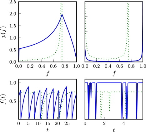
Figure 5.

(Top panels) Examples of steady-state fitness distribution p(f) for parameter values Δγ = 0.1 (left) and 100 (right); other parameters are λ = 0, kB = 0.5, ξ = 1, α = −0.99, and f∗ = 0.75. In each plot, the solid line corresponds to a value of kA = 0 (no switching), whereas the dashed plot is for kA = kA∗ (switching rate given by Eq. 19). (Bottom panels) Examples of fitness trajectories corresponding to the parameter values of the top panel.
