Dynamic Data-Driven Finite Element Models for Laser Treatment of Cancer

Abstract

Elevating the temperature of cancerous cells is known to increase their susceptibility to subsequent radiation or chemotherapy treatments, and in the case in which a tumor exists as a well-defined region, higher intensity heat sources may be used to ablate the tissue. These facts are the basis for hyperthermia based cancer treatments. Of the many available modalities for delivering the heat source, the application of a laser heat source under the guidance of real-time treatment data has the potential to provide unprecedented control over the outcome of the treatment process [7, 18]. The goals of this work are to provide a precise mathematical framework for the real-time finite element solution of the problems of calibration, optimal heat source control, and goal-oriented error estimation applied to the equations of bioheat transfer and demonstrate that current finite element technology, parallel computer architecture, data transfer infrastructure, and thermal imaging modalities are capable of inducing a precise computer controlled temperature field within the biological domain.

1 Introduction

Today, cancer is the second most common cause of death in the United States. In 2006, about 564,830 Americans are expected to die of cancer. Among the most common forms of the disease are cancer of the prostate and breast, accounting for 10% and 15% of all cancer related deaths in men and women, respectively. Current detection technology has led to a 5-year relative survival rate of greater than 90% for prostate and breast cancer [4]. Given these survival rates, the quality of life of the patient post-treatment is a very important factor. Traditional medical treatment of early stage prostate and breast cancer, including radical prostatectomy, pelvic lymphadenectomy, lumpectomy, and mastectomy are major surgical procedures and are associated with many surgical complications. Ablation therapies delivered under various treatment modalities are a very promising, minimally invasive, alternative to standard treatment and show significant potential as an effective cancer treatment to eradicate the disease while maintaining functionality of infected organs and minimizing complications and relapse.

The physical basis for thermal therapies is that exposing cells to temperatures outside their natural environment for certain periods of time can damage and even destroy the cells. However, one of the limiting factors in all forms of ablation therapy, including cryotherapy, microwave, radio-frequency, and laser, is the ability to control the energy deposition to prevent damage to adjacent healthy tissue [19].

Recent advances in imaging technology allow the imaging of the geometry of tissue and an overlaying temperature field using MRI and new MRTI technology. MRTI has the desirable properties of excellent soft-tissue contrast, the ability to provide fast, quantitative temperature imaging in a variety of tissues, and the capability of providing biologically relevant information regarding the extent of injury immediately following therapy [5]. Image guidance [18, 20] has the potential to facilitate unprecedented control over bioheat transfer by providing real time treatment monitoring through temperature feedback during treatment delivery. A similar idea using ultrasound guided cryotherapy has been studied and shows good results [19]. However, the hypothermic regime requires temperature differentials of 70° from normothermia to ablate the tissue. Tissue ablation in the hyperthermic regime requires substantially less energy deposition, temperature differentials of 10°, suggesting that MRTI guidance under laser therapy could provide superior control over the bioheat transfer.

The goal of this work is to deliver a computational model of bioheat transfer that employs real-time, patient specific data and provides real-time high fidelity predictions to be used concomitantly by the surgeon in the laser treatment process. The model employs an adaptive hp-finite element approximation of the nonlinear parabolic Pennes equation and uses adjoint-based algorithms for inverse analysis, model calibration, and adaptive control of cell damage. The target disease of this research are localized adenocarcinomas of the breast, prostate, cerebrum, and other tissues in which a well-defined tumor may form. The algorithms developed also provide a potentially viable option to treat other parts of the anatomy in patients with more advanced and aggressive forms of cancer who have reached their limit of radiation and chemotherapy treatment.

The adaptive data driven computational control system for controlling laser treatment of prostate cancer described is an example of a Dynamic-Data-Driven Applications System (DDDAS) in which simulation models interact with measurement devices and assimilate data over a computational grid for the purpose of producing high-fidelity predictions of physical events.

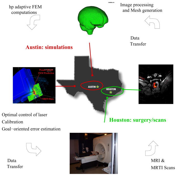
The development stages uses canines as the host of prostate and brain tumors. The actual laboratory at M.D. Anderson Cancer Center in Houston, TX is connected through a computational grid to the computing center in Austin, TX. Prior to treatment, MRI data is used to generate a finite element mesh of the patient-specific biological domain. The mesh is then optimized to a particular quantity of interest using goal-oriented estimation and adaption. The tool then proceeds to solve an optimal control problem, wherein the laser parameters (location of optical fiber, laser power, etc.) are controlled to eliminate/sensitize cancer cells, minimize damage to healthy cells, and control Heat Shock Protein (HSP) expression. Upon initiation of the treatment process, real-time MRI data is employed to co-register the computational domain and MRTI data is used to calibrate the bioheat transfer model to the biological tissue values of the patient. As new data is given intermittently, computation is compared to the measurements of the real-time treatment and an appropriate course of action is chosen according to the differences seen. A parallel computing paradigm is used to meet the demands of rapid calibration and adapting the computational mesh and models to control approximation and modeling error. From a computational point of view, the orchestration of a successful laser treatment is to solve the problems of co-registration, calibration, optimal control, and mesh refinement invisibly to the surgeon, and merely provide the surgeon with an interface to the optimal laser parameters during treatment. A schematic of the control loop is shown in Figure 1. The mathematical characterization of so-called HSP expression is also described as are laboratory procedures for measuring tissue damage, mesh generation, and the development of the computational infrastructure for calibration procedures, verification and validation procedures, and inverse modeling and sensitivity analysis.

Fig. 1.

The Control Loop.

2 Mesh Generation

The first step in simulation is to construct a finite element mesh used for the governing bioheat transfer equations. The mesh generation involves two steps: (1) construction, from MRI data, of a finite element mesh to represent the geometry and (2) overlaying the MRTI temperature field onto the finite element mesh.

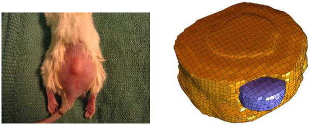
As an initial test of the imaging system when employed in experiments with laboratory animals, we first consider data pertaining to a mouse. A sample of the MRI data used to construct a mesh of the mouse and tumor is shown in Figure 3. In the case of prostate cancer, prostate tumor cells were inoculated in the hind legs of a mouse and grown to a tumor burden of less than 1.0 cc, Figure 2. The hexahedral mesh of the tumor (blue) and tissue (yellow), shown in Figure 2, was created by a semi-automatic segmentation method adapted to find the interface boundaries of tumor and tissue. Cubic spline and lofting methods are applied to obtain smooth boundaries from the segmented MRI data [16, 21].

Fig. 3.

MRI Data of Mouse

Fig. 2.

Mouse and Mesh (from [16])

2.1 MRTI Data-Filtering

Spatio-temporal temperature distribution is measured during the laser treatment with update times less than 6 seconds per image and thickness between planes of 3.5 mm. The temperature field, measured in the biological domain, is first filtered to eliminate any noise and then nodal temperature values are assigned to the mesh by taking the interpolant of the MRTI temperature data.

3 HSP Characterization and Damage Model

Heat shock proteins are a latent defense mechanism built into all cells, including cancer cells, that provide enhanced viability of tumor tissue indirectly by preventing a damaged cell from going into apoptosis, resulting in the recurrence of cancer. Knowledge of temperature history versus time during treatment has been used to predict thermal necrosis in regions where damage is severe, but in regions where temperatures are insufficient to coagulate proteins, the results and subsequent effects have been difficult to predict. This is due, in part, to the expression of heat shock protein (HSP) in the regions of thermal stress. Consequently, knowledge of the thermal dose necessary to activate or de-activate HSP expression as a function of temperature and time in the affected tissue [16, 15] can be critical in planning and implementing an effective thermal treatment by laser surgery.

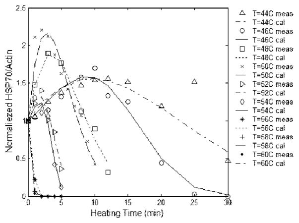
Heat Shock Proteins are a family of gene products expressed in higher concentrations in the presence of environmental stresses. The name vastly understates the HSP family’s astounding versatility. These proteins have been identified as critical components of cell survival under adverse environmental conditions. Various levels of HSP species indicate the health or likelihood of cell proliferation or drug resistance. Also, measures of cell damage as a function of temperature and time for a specific patient is a critical indication of the effectiveness of thermo-therapies. Knowledge of the temperatures necessary to elicit interaction in tumor resistance and cell damage is essential to effectively produce a desired tissue response and surgical outcome. The work of Rylander [15] developed a model for HSP expression and cell damage based on an Arrhenius model for a mouse. Figure 4 shows the comparison of the experimentally determined HSP expression with the predicted values of (1). An empirical formula for the concentration of HSP expression, $H(u,t)\left[\frac{mg}{ml}\right]$, at temperature, u, and time, t, based on laboratory tests is [15]:

$$H(u,t)=H_0{e}^{\alpha t-\beta t^{\gamma }}$$ (1)

where α, β, and γ are time independent parameters that may depend on temperature, with γ > 1.

Fig. 4.

HSP Expression Model

Cellular damage is measured in terms of the damage fraction F_D predicted by means of an Arrhenius integral formulation [16].

$$F_D(\mathbf{x},t)=1-e^{-\mathrm{\Omega }(\mathbf{x},t)}\mathrm{\Omega }(\mathbf{x},t)=ln(C_0/C_t)=A{\int }_0^t{e}^{\frac{E_a}{Ru(\mathbf{x},\tau )}}d\tau$$ (2)

where C₀ is the initial concentration of healthy cells, C_t the concentration of healthy cells after heating at time t, A the pre-exponential scaling factor, E_a the activation energy of the injury process, R the universal gas constant, and u the absolute temperature.

4 Bioheat Transfer Model

Driving the prediction of the HSP and cellular damage is the temperature field produced by the well-known Pennes bioheat transfer model [13]. Liu [6] has shown Pennes model [13] to give good results for prediction of temperature field in the prostate. The formal statement of Pennes bioheat model is as follows

Find the spatially and temporally varying temperature field u (x, t) such that

$$\rho c_p\frac{\partial u}{\partial t}-\nabla ·(k(u)\nabla u)+\omega (u)c_{\mathit{blood}}(u-u_a)=Q_{\mathit{laser}}(\mathbf{x},t)\text{in}\mathrm{\Omega }$$

given the Cauchy and Neumann boundary conditions

$$\begin{array}{c}-k(u)\nabla u·\mathbf{n}=h(u-u_{\infty })\text{on}\partial {\mathrm{\Omega }}_C\\ -k(u)\nabla u·\mathbf{n}=\mathcal{G}\text{on}\partial {\mathrm{\Omega }}_N\end{array}$$

and the initial condition

$$u(\mathbf{x},0)=u^0\text{in}\mathrm{\Omega }$$

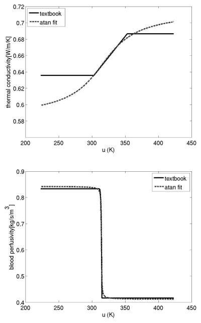
Here $k\left[\frac{J}{s·m·K}\right]$ and $\omega \left[\frac{kg}{s{m}^3}\right]$ are bounded functions of u, determined empirically to be of the form

$$\begin{array}{l}k(u)=k_0+k_1\text{atan}({\stackrel{\sim }{k}}_2(u-{\widehat{k}}_3))\\ \omega (u)={\omega }_0+{\omega }_1\text{atan}({\stackrel{\sim }{\omega }}_2(u-{\widehat{\omega }}_3))\end{array}$$

c_p and c_blood are the specific heats, u_a the arterial temperature, ρ is the density, and h is the coefficient of cooling. The laser source term Q_laser is a linear function of laser power and exhibits exponential decay with distance from the source.

$$\begin{array}{l}{Q}_{\mathit{laser}}(\mathbf{x},t)=3P(t){\mu }_a{\mu }_{tr}\frac{exp(-{\mu }_{\mathit{eff}}||\mathbf{x}-{\mathbf{x}}_0||)}{4\pi \left|\right|\mathbf{x}-{\mathbf{x}}_0\left|\right|}\\ {\mu }_{tr}={\mu }_a+{\mu }_s(1-\gamma ){\mu }_{\mathit{eff}}=\sqrt{3{\mu }_a{\mu }_{tr}}\end{array}$$

P = is the laser power, μ_a, μ_s = are laser coefficients related to laser wavelength and give probability of absorption of photons by tissue, γ is the anisotropy factor, and x₀ = is the position of laser photon source. Tables 1 and 2 contain constitutive data from the work of Rylander [17].

Table 1.

Model Coefficients (From Rylander [17])

Laser Wavelength	810 nm	μs	14.74cm	μa	0.046 cm	ρtissue	$1045\frac{kg}{m^3}$
ua	310 K	ρblood	$1058\frac{kg}{m^3}$	$c_p^{\mathit{blood}}$	$3840\frac{J}{kg·K}$	$c_p^{\mathit{tissue}}$	$3600\frac{J}{kg·K}$

Table 2.

Model Coefficients

k(u) = k0 + k1 · atan(k2(u− k3))		ω(u) =ω0 + ω1 · atan(ω2(u − ω3))
k0	$0.6489\left[\frac{J}{s·m·K}\right]$	ω0	$0.6267\left[\frac{kg}{s{m}^3}\right]$
k1	$0.0427\left[\frac{J}{s·m·K}\right]$	ω1	$-0.137\left[\frac{kg}{s{m}^3}\right]$
k2	$0.0252\left[\frac{1}{K}\right]$	ω2	$2.3589\left[\frac{1}{K}\right]$
k3	315.314 [K]	ω3	314.262 [K]

Our weak form of the Pennes bioheat transfer model is as follows:

Given a set of model, β, and laser, η, parameters,

Find u (x, t) ∈ ≡ H¹([0, T], H¹(Ω)) s.t.

B(u, β; v) = F(η; v)   ∀v ∈

where the explicit functional dependence on the model parameters, β = (k₀, k₁, k̃₃, k̂₃, ω₀(x), ω₁, ω̃₃, ω̂₃), and laser parameters, η= (P(t), x₀, μ_a, μ_s), expressed as follows

$$\begin{array}{l}B(u,\beta ;v)={\int }_0^T{\int }_{\mathrm{\Omega }}\left[\rho c_p\frac{\partial u}{\partial t}v+k(u,\beta )\nabla u·\nabla v+\omega (u,\beta )c_{\mathit{blood}}(u-u_a)v\right]\mathit{dxdt}\\ +{\int }_0^T{\int }_{\partial {\mathrm{\Omega }}_C}huv\mathit{dAdt}+{\int }_{\mathrm{\Omega }}u(\mathbf{x},0)v(\mathbf{x},0)dx\end{array}$$ (3)

$$F(\eta ;v)={\int }_0^T{\int }_{\mathrm{\Omega }}{Q}_{\mathit{laser}}(\mathbf{x},\eta )v\mathit{dxdt}+{\int }_0^T{\int }_{\partial {\mathrm{\Omega }}_C}h{u}_{\infty }v\mathit{dAdt}-{\int }_0^T{\int }_{\partial {\mathrm{\Omega }}_N}\mathcal{G}v\mathit{dAdt}+{\int }_{\mathrm{\Omega }}{u}^{0}v(\mathbf{x},0)dx$$ (4)

4.1 Calibration, Optimal Control

The control loop involves three major problems: calibration of the Pennes model to patient specific MRTI data, optimal positioning and power supply of the laser heat source, and computing goal oriented error estimates. Each of these problems is formally stated below.

The problem of model calibration is to find the set of thermal conductivity parameters k₀, k₁, k̃₃, k̂₃, and blood perfusivity parameters ω₀(x), ω₁, ω̃₃, ω̂₃ that minimize the norm of the difference between the predicted temperature field and the experimentally determined temperature field at each time instance of the experimental data. ω₀(x) is allowed to vary over the spatial dimension as the blood perfusivity within the necrotic core of a cancerous tumor is expected to be significantly lower than the surrounding healthy tissue. The calibration problem may be stated as follows:

Given a set of laser parameters, η ₀, and an experimentally determined temperature field at time instances t_n, n = 1, 2, … N_exp within the region Ω_χ ⊂ Ω

$$u_{\mathit{exp}}(\mathbf{x},t_n)\mathbf{x}\in {\mathrm{\Omega }}_{\chi }$$

find the best combination of model coefficients, β^* ∈ ℙ, that produces the temperature field, u^* ∈ , such that

$$Q(u^{\ast }({\eta }_0,{\beta }^{\ast }),{\beta }^{\ast })=\frac{1}{2}{\int }_0^T{\int }_{\mathrm{\Omega }}\chi (\mathbf{x}){(u^{\ast }(\mathbf{x},t)-u_{\mathit{exp}}(\mathbf{x},t))}^2\mathit{dxdt}+\frac{\gamma }{2}{\int }_{\mathrm{\Omega }}\nabla {\omega }_0^{\ast }(\mathbf{x})·\nabla {\omega }_0^{\ast }(\mathbf{x})dx$$

satisfies

$$\begin{array}{l}Q(u^{\ast }({\eta }_0,{\beta }^{\ast }),{\beta }^{\ast })=\underset{\beta \in \mathbb{P}}{inf}Q(u({\eta }_0,\beta ),\beta )\\ \mathbb{P}=\{\beta \in {ℝ}^4\times C^1(\mathrm{\Omega })\times {ℝ}^3:\exists !u\text{s}.\text{t}.B(u,\beta ;v)=F({\eta }_0,v)\forall v\in \mathcal{V}\}\end{array}$$

The problem of optimal laser heating control is to find the position, x₀, power, P (t), and laser frequency μ_a, μ_s that maximizes damage to the cancerous tissue while minimizing damage to healthy tissue in some metric. The metric shown here is the ℒ² ([0, T ]; ℒ²(Ω)) norm of the difference between the computed solution and an ’ideal’ temperature field. Other metrics may be the ℒ²(Ω) norm of the difference between the computed damage fraction, equation (2), and an ideal damage field within the biological domain at the end of the treatment process or the ℒ² ([0, T]; ℒ²(Ω)) norm of the difference between the computed HSP expression field, equation (1), and an ideal HSP expression field.

$${\left|\right|F_D(\mathbf{x},T)-F_D^{\mathit{ideal}}(\mathbf{x})\left|\right|}_{{\mathcal{L}}^2(\mathrm{\Omega })}^2{\left|\right|H-H^{\mathit{ideal}}\left|\right|}_{{\mathcal{L}}^2([0,T];{\mathcal{L}}^2(\mathrm{\Omega }))}^2$$

Optimal control of the laser source term is stated as:

Given a set of model coefficients, β ₀, and the ideal temperature field that maximizes damage to cancerous tissue while minimizing damage to healthy tissue

$$\phi (\mathbf{x})\equiv \{\begin{array}{ll}{37.0}^{o}C\hfill & \mathbf{x}\in {\mathrm{\Omega }}_H\hfill \\ {50.0}^{o}C\hfill & \mathbf{x}\in {\mathrm{\Omega }}_C\hfill \end{array}$$

where Ω_H and Ω_C are the domains of the healthy and cancerous tissue respectively, find the best combination of laser position and power, η^* ∈ ℙ, that produces the temperature field, u^* ∈ , such that

$$Q(u^{\ast }({\eta }^{\ast },{\beta }_0),{\eta }^{\ast })=\frac{1}{2}{\left|\right|u-\phi \left|\right|}_{{\mathcal{L}}^2([0,T];{\mathcal{L}}^2(\mathrm{\Omega }))}^2=\frac{1}{2}{\int }_0^T{\int }_{\mathrm{\Omega }}{(u^{\ast }(\mathbf{x},t)-\phi (\mathbf{x}))}^2\mathit{dxdt}$$ (5)

satisfies

$$\begin{array}{l}Q(u^{\ast }({\eta }^{\ast },{\beta }_0),{\eta }^{\ast })=\underset{\eta \in \mathbb{P}}{inf}Q(u(\eta ,{\beta }_0),\eta )\\ \mathbb{P}=\{\eta \in C^0([0,T])\times {ℝ}^5:\exists !u\text{s}.\text{t}.B(u,{\beta }_0;v)=F(\eta ;v)v\in \mathcal{V}\}\end{array}$$

where is the appropriate space for the bioheat transfer model.

4.2 Mesh Refinement

Goal oriented error estimates [9] are calculated under the following framework:

• Fixing the parameters β₀ and η₀ denote

$$C(u;v)=B(u,{\beta }_0;v)-F({\eta }_0;v)$$

• Let and represent two finite dimensional spaces such that ⊂ .

• ||u^hp − u|| ≤ || u^h −u|| where u, u^h, u^hp satisfy the Pennes model constraints

$$\begin{array}{c}C(u;v)=0\forall v\in \mathcal{V}\\ C(u^{hp};v^{hp})=0\forall v^{hp}\in {\mathcal{V}}^{hp}\\ C(u^h;v^h)=0\forall v^h\in {\mathcal{V}}^h\end{array}$$

We presume that the solution u^hp ∈ is a more accurate representation of the exact solution u ∈ than u^h ∈ ⊂ ; likewise an arbitrary quantity of interest, Q, evaluated at Q(u^hp) is a more accurate representation of Q(u) than the quantity of interest evaluated at Q(u^h). As an explicit example, consider the quantity of interest to be an averaged value of the temperature in a domain defined through the characteristic function, χ(x),

$$Q(u({\eta }_0,{\beta }_0))=\frac{1}{2}{\left|\right|\chi (\mathbf{x})u(\mathbf{x},t)\left|\right|}_{{\mathcal{L}}^2([0,\tau ];{\mathcal{L}}^2(\mathrm{\Omega }))}^2$$

Using the following Taylor series approximations,

$$\begin{array}{l}Q(u^{hp})\approx Q(u^h)+\delta Q(u^h;u^{hp}-u^h)\\ C(u^{hp};v^{hp})\approx C(u^h;v^{hp})+\delta C(u^h;u^{hp}-u^h,v^{hp})\end{array}$$

with

$$\begin{array}{l}\delta Q(u;\widehat{u})\equiv \underset{\theta \to 0}{lim}\frac{1}{\theta }[Q(u+\widehat{u})-Q(u)]\\ \delta C(u;\widehat{u};v)\equiv \underset{\theta \to 0}{lim}[C(u+\widehat{u};v)-C(u;v)]\end{array}$$

we may solve for the adjoint variable p^hp ∈ such that

$$\delta Q(u^h;\widehat{u})=\delta C(u^h;\widehat{u},p^{hp})\forall \widehat{u}\in {\mathcal{V}}^{hp}$$

Then

$$\begin{array}{l}Q(u^{hp})-Q(u^h)=-C(u^h,p^{hp})=F(p^{hp})-B(u^h;p^{hp})\\ =-{\int }_0^T{\int }_{\mathrm{\Omega }}\left[\rho c_p\frac{\partial u^h}{\partial t}{p}^{hp}+k(u^h,{\beta }_0)\nabla u^h·\nabla p^{hp}+\omega (u^h,{\beta }_0)c_{\mathit{blood}}(u^h-u_a)p^{hp}\right]\mathit{dxdt}\\ -{\int }_0^T{\int }_{\partial {\mathrm{\Omega }}_C}h(u^h-u_{\infty })p^{hp}\mathit{dAdt}-{\int }_0^T{\int }_{\partial {\mathrm{\Omega }}_N}\mathcal{G}{p}^{hp}\mathit{dAdt}+{\int }_0^T{\int }_{\mathrm{\Omega }}{Q}_{\mathit{laser}}(\mathbf{x},{\eta }_0)p^{hp}\mathit{dxdt}\\ ={\int }_0^T\mathcal{Z}(t)dt={\int }_{\mathrm{\Omega }}\mathcal{X}(\mathbf{x})dx+{\int }_{\partial {\mathrm{\Omega }}_C}\mathcal{R}(\mathbf{x})dA+{\int }_{\partial {\mathrm{\Omega }}_N}\mathcal{N}(\mathbf{x})dA\end{array}$$

Where (t) is defined as

$$\begin{array}{l}\mathcal{Z}(t)=-{\int }_{\mathrm{\Omega }}\left[\rho c_p\frac{\partial u^h}{\partial t}{p}^{hp}+k(u^h,{\beta }_0)\nabla u^h·\nabla p^{hp}+\omega (u^h,{\beta }_0)c_{\mathit{blood}}(u^h-u_a)p^{hp}\right]dx\\ -{\int }_{\partial {\mathrm{\Omega }}_C}h(u^h-u_{\infty })p^{hp}dA-{\int }_{\partial {\mathrm{\Omega }}_N}\mathcal{G}{p}^{hp}dA+{\int }_{\mathrm{\Omega }}{Q}_{\mathit{laser}}(\mathbf{x},{\eta }_0)p^{hp}dx\end{array}$$

This quantity may be used to determine when greater time stepping accuracy is needed. (x), ℛ(x), and (x) defined as

$$\begin{array}{l}\mathcal{X}(\mathbf{x})={\int }_0^T{Q}_{\mathit{laser}}(\mathbf{x},{\eta }_0)p^{hp}-\rho c_p\frac{\partial u^h}{\partial t}{p}^{hp}-k(u^h,{\beta }_0)\nabla u^h·\nabla p^{hp}-\omega (u^h,{\beta }_0)c_{\mathit{blood}}(u^h-u_a)p^{hp}dt\\ \mathcal{R}(\mathbf{x})=-{\int }_0^{T}h(u^h-u_{\infty })p^{hp}dt\mathcal{N}(\mathbf{x})=-{\int }_0^T\mathcal{G}{p}^{hp}dt\end{array}$$

may be used to determine when spatial mesh refinement is needed.

4.3 Optimization Framework

The calibration and optimal control problems in the control loop may be posed as the following optimization problem

Find q^* ∈ ℙ s.t.

$$Q(u(q^{\ast }),q^{\ast })=\underset{q\in \mathbb{P}}{inf}Q(u(q),q)$$

where q is a parameter in the control space ℙ,

$$\mathbb{P}\equiv \left\{\begin{array}{cc}q\text{such}\text{that}& \\ \exists !u\in \mathcal{V}:C(u,q;v)=0& \forall v\in \mathcal{V}\end{array}\right\}$$

and u is the state variable determined by a variational PDE of the form

$$C(u,q;v)=B(u,q;v)-F(q;v)=0\forall v\in \mathcal{V}$$

in the appropriate Hilbert space, .

The demands of real-time computation will only permit the computation of the following Gateaux derivative, δQ, of the objective function.

$$\delta Q(q,\widehat{q})\equiv \underset{\theta \to 0}{lim}\frac{1}{\theta }[Q(u(q+\theta \widehat{q}),q+\theta \widehat{q})-Q(u(q),q)]$$

The gradient is computed by the adjoint method under the assumptions that the solution, objective function, and constraints admit the following Taylor series expansions.

$$\begin{array}{l}u(q+\theta \widehat{q})=u(q)+\theta u^{\prime }(q;\widehat{q})+{\theta }^2(\dots )\\ Q(u+\theta \widehat{u},q+\theta \widehat{q})=Q(u,q)+\theta {\delta }_{u}Q(u,q;\widehat{u})+\theta {\delta }_{q}Q(u,q;\widehat{q})+{\theta }^2(\dots )\\ C(u+\theta \widehat{u},q+\theta \widehat{q};v)=C(u,q;v)+\theta {\delta }_{u}C(u,q;\widehat{u};v)+\theta {\delta }_{q}C(u,q;\widehat{q};v)+{\theta }^2(\dots )\end{array}$$

where the Gateaux derivatives are defined below.

$$\begin{array}{c}{u}^{\prime }(q;\widehat{q})\equiv \underset{\theta \to 0}{lim}\frac{1}{\theta }[u(q+\theta \widehat{q})-u(q)]\\ {\delta }_{u}Q(u,q;\widehat{u})\equiv \underset{\theta \to 0}{lim}\frac{1}{\theta }[Q(u+\widehat{u},q)-Q(u,q)]\\ {\delta }_{q}Q(u,q;\widehat{q})\equiv \underset{\theta \to 0}{lim}\frac{1}{\theta }[Q(u,q+\widehat{q})-Q(u,q)]\\ {\delta }_{u}C(u,q;\widehat{u};v)\equiv \underset{\theta \to 0}{lim}[C(u+\widehat{u},q;v)-C(u,q;v)]\\ {\delta }_{q}C(u,q;\widehat{q};v)\equiv \underset{\theta \to 0}{lim}[C(u,q+\widehat{q};v)-C(u,q;v)]\end{array}$$

Theorem

Given q ∈ ℙ, (and hence u ∈ by definition), the derivative of the objective function is

δQ(q,q̂) = δ_qQ(u(q),q; q̂) − δ_qC(u(q),q; q̂, p)

where p ∈ is the solution to the adjoint problem.

Find p ∈ :

δ_uC(u(q),q; û;, p) = δ_uQ(u(q),q; û)   ∀û ∊

Proof

The solution to the adjoint problem, p, implies that

$${\delta }_{u}C(u(q),q;u^{\prime }(q;\widehat{q});p)={\delta }_{u}Q(u(q),q;u^{\prime }(q;\widehat{q}))\forall \widehat{q}\in \mathbb{P}$$

from the first variation of the PDE constraints we have that

$${\delta }_{u}C(u(q),q;u^{\prime }(q;\widehat{q});p)=-{\delta }_{q}C(u(q),q;\widehat{q};p)$$

the solution follows

$$\begin{array}{l}\delta Q(q,\widehat{q})={\delta }_{u}Q(u(q),q;u^{\prime }(q;\widehat{q}))+{\delta }_{q}Q(u(q),q;\widehat{q})\\ ={\delta }_{q}Q(u(q),q;\widehat{q})-{\delta }_{q}C(u(q),q;\widehat{q};p)\end{array}$$

The following Taylor series expansion are used in computing the Gateaux derivatives of the variational form of Pennes model:

$$\begin{array}{l}k(u+\theta \widehat{u},\beta +\theta \widehat{\beta })=k(u,\beta )+\theta \widehat{u}\frac{\partial k}{\partial u}+\theta {\widehat{k}}_0\frac{\partial k}{\partial k_0}+\theta {\widehat{k}}_1\frac{\partial k}{\partial k_1}+\theta {\widehat{k}}_2\frac{\partial k}{\partial k_2}+\theta {\widehat{k}}_3\frac{\partial k}{\partial k_3}+{\theta }^2(\dots )\\ \omega (u+\theta \widehat{u},\beta +\theta \widehat{\beta })=\omega (u,\beta )+\theta \widehat{u}\frac{\partial \omega }{\partial u}+\theta {\widehat{\omega }}_0\frac{\partial \omega }{\partial {\omega }_0}+\theta {\widehat{\omega }}_1\frac{\partial \omega }{\partial {\omega }_1}+\theta {\widehat{\omega }}_2\frac{\partial \omega }{\partial {\omega }_2}+\theta {\widehat{\omega }}_3\frac{\partial \omega }{\partial {\omega }_3}{\theta }^2(\dots )\end{array}$$

Notice that the variational form of the adjoint problem for the calibration, optimal control, and goal oriented error estimates are all the same:

$$\begin{array}{l}{\delta }_{u}C(u,\beta ;\widehat{u},p)={\delta }_{u}B(u,\beta ;\widehat{u},p)={\int }_0^T{\int }_{\mathrm{\Omega }}-\rho c_p\frac{\partial p}{\partial t}\widehat{u}\mathit{dxdt}+{\int }_0^T{\int }_{\mathrm{\Omega }}k(u,\beta )\nabla \widehat{u}·\nabla p+\widehat{u}\frac{\partial k}{\partial u}\nabla u·\nabla p\mathit{dxdt}\\ +{\int }_0^T{\int }_{\mathrm{\Omega }}\omega (u,\beta )\widehat{u}p+\widehat{u}\frac{\partial \omega }{\partial u}(u-u_a)p\mathit{dxdt}+{\int }_{\mathrm{\Omega }}\widehat{u}(\mathbf{x},T)p(\mathbf{x},T)dx+{\int }_0^T{\int }_{\partial \mathrm{\Omega }}h\widehat{u}p\mathit{dAdt}\end{array}$$

where the only difference is source term δ_uQ(u(q), q; û) which depends on the quantity of interest. The strong form of the adjoint formulation is as follows:

Given the spatially and temporally varying temperature field u (x, t) find the Lagrange multiplier p(x, t) such that

$$\begin{array}{l}-\rho c_p\frac{\partial p}{\partial t}-\nabla ·(k(u)\nabla p)+\frac{\partial k}{\partial u}(u,\beta )\nabla u·\nabla p+\omega (u,\beta )p\\ +\frac{\partial \omega }{\partial u}(u,\beta )p(u-u_a)=\{\begin{array}{rr}\hfill u-u_{\mathit{exp}}(\mathbf{x},t)(\text{calibration})& \hfill \\ \hfill u-\phi (\mathbf{x})(\text{optimal}\text{control})& \hfill \text{in}\mathrm{\Omega }\\ \hfill \chi (\mathbf{x})u(\text{error}\text{estimate})& \hfill \end{array}\end{array}$$

given the boundary conditions

$$\begin{array}{c}-k(u)\nabla p·\mathbf{n}=hp\text{on}\partial {\mathrm{\Omega }}_C\\ -k(u)\nabla p·\mathbf{n}=0\text{on}\partial {\mathrm{\Omega }}_N\end{array}$$

and the terminal condition

$$p(\mathbf{x},T)=0\text{in}\mathrm{\Omega }$$

When approximations of the temperature field, u(x, t), and the adjoint variable, p(x, t), are known, the first variation of the quantity of interest for the calibration problem may be obtained explicitly as follows.

$$\delta Q(\beta ,\widehat{\beta })=\left[\begin{array}{l}-{\int }_0^T{\int }_{\mathrm{\Omega }}\nabla u·\nabla p{\widehat{k}}_0\mathit{dxdt}\hfill \\ -{\int }_0^T{\int }_{\mathrm{\Omega }}\text{atan}(k_2(u-k_3))\nabla u·\nabla p{\widehat{k}}_1\mathit{dxdt}\hfill \\ -{\int }_0^T{\int }_{\mathrm{\Omega }}\frac{k_1(u-k_3)}{1+k_2^2{(u-k_3)}^2}\nabla u·\nabla p{\widehat{k}}_2\mathit{dxdt}\hfill \\ -{\int }_0^T{\int }_{\mathrm{\Omega }}\frac{-k_1{k}_2}{1+k_2^2{(u-k_3)}^2}\nabla u·\nabla p{\widehat{k}}_3\mathit{dxdt}\hfill \\ -{\int }_0^T{\int }_{\mathrm{\Omega }}(u-u_a)p{\widehat{\omega }}_0(\mathbf{x})\mathit{dxdt}+{\int }_{\mathrm{\Omega }}{\omega }_0(\mathbf{x}){\widehat{\omega }}_0(\mathbf{x})dx\hfill \\ -{\int }_0^T{\int }_{\mathrm{\Omega }}\text{atan}({\omega }_2(u-{\omega }_3))(u-u_a)p{\widehat{\omega }}_1\mathit{dxdt}\hfill \\ -{\int }_0^T{\int }_{\mathrm{\Omega }}\frac{{\omega }_1(u-{\omega }_3)}{1+{\omega }_2^2(u-{\omega }_3)}(u-u_a)p{\widehat{\omega }}_2\mathit{dxdt}\hfill \\ -{\int }_0^T{\int }_{\mathrm{\Omega }}\frac{-{\omega }_1{\omega }_2}{1+{\omega }_2^2{(u-{\omega }_3)}^2}(u-u_a)p{\widehat{\omega }}_3\mathit{dxdt}\hfill \end{array}\right]$$

The first variation for the quantity of interest for optimal control is as follows:

$$\delta Q(\eta ,\widehat{\eta })=\left[\begin{array}{l}{\int }_0^T{\int }_{\mathrm{\Omega }}\frac{3{\mu }_a{\mu }_{tr}exp(-{\mu }_{\mathit{eff}}||\mathbf{x}-{\mathbf{x}}_0||)}{4\pi \left|\right|\mathbf{x}-{\mathbf{x}}_0\left|\right|}p\widehat{P}(t)\mathit{dxdt}\hfill \\ {\int }_0^T{\int }_{\mathrm{\Omega }}3P(t)\frac{exp(-{\mu }_{\mathit{eff}}||\mathbf{x}-{\mathbf{x}}_0||)}{4\pi \left|\right|\mathbf{x}-{\mathbf{x}}_0\left|\right|}\left({\mu }_{tr}+{\mu }_a-{\mu }_{tr}{\mu }_a\left|\right|\mathbf{x}-{\mathbf{x}}_0\left|\right|\frac{3({\mu }_a+{\mu }_{tr})}{2{\mu }_{\mathit{eff}}}\right)p{\widehat{\mu }}_a\mathit{dxdt}\hfill \\ {\int }_0^T{\int }_{\mathrm{\Omega }}3P(t)\frac{exp(-{\mu }_{\mathit{eff}}||\mathbf{x}-{\mathbf{x}}_0||)}{4\pi \left|\right|\mathbf{x}-{\mathbf{x}}_0\left|\right|}\left({\mu }_a-{\mu }_{tr}{\mu }_a\left|\right|\mathbf{x}-{\mathbf{x}}_0\left|\right|\frac{3({\mu }_a(1-\gamma ))}{2{\mu }_{\mathit{eff}}}\right)p{\widehat{\mu }}_s\mathit{dxdt}\hfill \\ {\int }_0^T{\int }_{\mathrm{\Omega }}3P(t){\mu }_a{\mu }_{tr}({\mu }_{\mathit{eff}}||\mathbf{x}-{\mathbf{x}}_0||+1)\frac{exp(-{\mu }_{\mathit{eff}}||\mathbf{x}-{\mathbf{x}}_0||)}{4\pi {\left|\right|\mathbf{x}-{\mathbf{x}}_0\left|\right|}^3}(x-x_0)p{\widehat{x}}_0\mathit{dxdt}\hfill \\ {\int }_0^T{\int }_{\mathrm{\Omega }}3P(t){\mu }_a{\mu }_{tr}({\mu }_{\mathit{eff}}||\mathbf{x}-{\mathbf{x}}_0||+1)\frac{exp(-{\mu }_{\mathit{eff}}||\mathbf{x}-{\mathbf{x}}_0||)}{4\pi {\left|\right|\mathbf{x}-{\mathbf{x}}_0\left|\right|}^3}(y-y_0)p{\widehat{y}}_0\mathit{dxdt}\hfill \\ {\int }_0^T{\int }_{\mathrm{\Omega }}3P(t){\mu }_a{\mu }_{tr}({\mu }_{\mathit{eff}}||\mathbf{x}-{\mathbf{x}}_0||+1)\frac{exp(-{\mu }_{\mathit{eff}}||\mathbf{x}-{\mathbf{x}}_0||)}{4\pi {\left|\right|\mathbf{x}-{\mathbf{x}}_0\left|\right|}^3}(z-z_0)p{\widehat{z}}_0\mathit{dxdt}\hfill \end{array}\right]$$

5 Results

Two main results are presented in this section. First, the overall computational feasibility of developing a laser treatment paradigm in which high performance computers control the bioheat data transferred from a remote site is demonstrated. Second, reliable computational predictions are shown when comparing results obtained using the Pennes model to the experimental MRTI data in canine cerebral tissue.

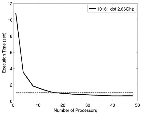
The typical time duration of a laser treatment is about five minutes. During a five minute span, one set of MRTI data is acquired every 6 seconds. The size of each set of MRTI data is ≈330kB (256×256×5 voxels) and the bandwidth of a commercial T1 Internet connection is ≈300kB/s. Accounting for connection latency, each set of MRTI data can be transferred between Houston and Austin in under two seconds. A finite element mesh consisting of approximately 10000 degrees of freedom is sufficient to resolve the geometry of the biological domain. The execution time of a representative 10 second bioheat transfer simulation is presented in Figure 6. The execution times represent 10 nonlinear state solves of Pennes model (10 one second time steps) combined with 10 linear adjoint solves to be used for calibration, optimal control, and/or error estimates. Computations were done at the Texas Advanced Computing Center on Dual-Core Linux Cluster. Each node of the cluster contains two Xeon Intel Duo-Core 64-bit processors (4 cores in all) on a single board, as an SMP unit. The core frequency is 2.66GHz and supports 4 floating-point operations per clock period. Each node contains 8GB of memory. The fastest time recorded is .67 seconds, meaning that in a real time 10 second span Pennes model can predict out to more than two minutes! Equivalently, in a 10 second times span roughly 14 corrections can be made to calibrate the model coefficients or optimize the laser parameters.

Fig. 6.

Executions times for a representative 10 second simulation (10 nonlinear state solve combined with 10 linear adjoint solve on 10000 dof system)

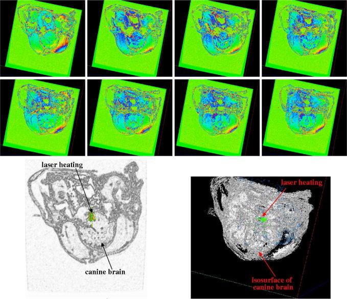
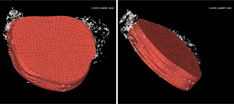
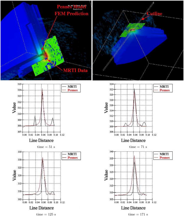
Preliminary computations comparing the predictions of Pennes model to experimental MRTI taken from a canine brain show very good agreement. A manual craniotomy of a canine skull was preformed to allow insertion of an interstitial laser fiber. Thirty-six two dimensional 256×256 pixels MRI images, Figure 7, of the canine brain were acquired. The field view was 200mm × 200mm with each image spaced 1mm apart. A finite element mesh of the biological domain generated from the MRI data is shown in Figure 8. The mesh consists of 8820 linear elements with a total of 9872 degrees of freedom. MRTI thermal imaging data was acquired in the form of five two dimensional 256×256 pixel images every six seconds for 120 time steps. The spacing between images was 3.5mm. The MRTI data was filtered then projected onto the finite element mesh. Figure 9 shows a cutline comparison between the MRTI data and the predictions of Pennes model. It is observed that the results delivered by the computational Pennes model slightly over diffuses the heat profile peaks compared to measured values. However, at early times the maximum temperature value is within 5% of the MRTI value.

Fig. 7.

Selected Slices of Canine MRI Brain Data and Iso-surface visualization of Canine MRI Brain Data

Fig. 8.

Finite Element Mesh of Canine MRI Brain Data

Fig. 9.

Cutline Comparison of MRTI Data to Pennes model predictions

6 Conclusion

Results indicate that adaptive hp-finite element technology implemented on parallel computer architectures and employing modern data transfer infrastructure and thermal imaging modalities are capable of predicting and guiding computer controlled temperature field within a biological domain at very good accuracies. Reliable finite element model simulations of laser therapies can be computed in a fraction of the time that the actual therapy takes place. These prediction capabilities combined with an understanding of HSP kinetics and damage mechanisms at the cellular and tissue levels due to thermal stress, together with recent advances for controlling discretization and modeling errors through adaptive control strategies combined with the modern methods of inverse analysis, calibration, uncertainty quantification, sensitivity analysis, and optimization [22, 12, 11, 14, 2, 8, 10, 9, 1, 3] provide a powerful methodology for planning and optimizing the delivery of thermo-therapy for cancer treatments. Moreover, from a computational point of view, changing the thermal delivery modality merely amounts to changing the source term in the governing PDE. This technology has the potential to be extended to many areas of thermal treatment including RF, microwave, ultrasound, and even cryotherapy applicators.

Fig. 5.

Comparison of arctan fit to text book values.

References

- 1.Bangerth W, Rannacher R. Adaptive Finite Element Methods for Solving Differential Equations. Birkhäuser; Verlag: 2003. [Google Scholar]
- 2.Becker Roland, Rannacher Rolf. An optimal control approach to a posteriori error estimation in finite element methods. Acta Numerica. 2001;10:1–102. [Google Scholar]
- 3.Braack M, Ern A. A posteriori control of modeling errors and discretization errors. Multiscale Model Simul. 2003;1:221–238. [Google Scholar]
- 4.American Cancer Society. Cancer Facts and Figures 2006. Atlanta: American Cancer Society; 2006. [Google Scholar]
- 5.Kangasniemi M, et al. Dynamic gadolinium uptake in thermally treated canine brain tissue and experimental cerebral tumors. Invest Radiol. 2003;38(2):102–107. doi: 10.1097/00004424-200302000-00005. [DOI] [PubMed] [Google Scholar]
- 6.Liu J, Zhu L, Xu L. Studies on the three-dimensional temperature transients in the canine prostate during transurethral microwave thermal therapy. J Biomech Engr. 2000;122:372–378. doi: 10.1115/1.1288208. [DOI] [PubMed] [Google Scholar]
- 7.McNichols RJ, et al. MR thermometry-based feedback control of laser interstitial thermal therapy at 980 nm. Lasers Surg Med. 2004;34(1):48–55. doi: 10.1002/lsm.10243. [DOI] [PubMed] [Google Scholar]
- 8.Oden JT, Prudhomme S. Goal-oriented error estimation and adaptavity for the finite element method. Computers and Mathematics with Applications. 2001;41(5–6):735–756. [Google Scholar]
- 9.Oden JT, Prudhomme S. Estimation of modeling error in computational mechanics. Journal of Computational Physics. 2002;182:496–515. [Google Scholar]
- 10.Oden JT, Prudhomme S, Hammerand DC, Kuczma MS. Modeling error and adaptivity in nonlinear continuum mechanics. Comput Meth Appl Mech Engrg. 2001;190:6663–6684. [Google Scholar]
- 11.Oden JT, Vemaganti K. Adaptive hierarchical modeling of heterogeneous structures. Predictability: quantifying uncertainty in models of complex phenomena. Phys D. 1999;133:404–415. [Google Scholar]
- 12.Oden JT, Zohdi Tarek I. Analysis and adaptive modeling of highly heterogeneous elastic structures. Comput Methods Appl Mech Eng. 1997;148(3–4):367–391. [Google Scholar]
- 13.Pennes HH. Analysis of tissue and arterial blood temperatures in the resting forearm. J Appl Physiol. 1948;1:93–122. doi: 10.1152/jappl.1948.1.2.93. [DOI] [PubMed] [Google Scholar]
- 14.Prudhomme Serge, Oden JT. On goal-oriented error estimation for elliptic problems: Applications to the control of pointwise errors. Comput Methods Appl Mech Eng. 1999;176:313–331. [Google Scholar]
- 15.Rylander MN, Feng Y, Diller KR. Thermally induced HSP 27, 60, and 70 expression kinetics and cell viability in normal and cancerous prostate cells. Cell Stress Chaperones. 2006 In review. [Google Scholar]
- 16.Rylander MN, Feng Y, Zhang J, Bass J, Hazle J, Diller K. Optimizing hsp expression in prostate cancer laser therapy through predictive computational models. J Biomed Optics. 2006 doi: 10.1117/1.2241310. In press. [DOI] [PubMed] [Google Scholar]
- 17.Rylander MN. PhD thesis. The University of Texas at Austin; 2005. Design of Hyperthermia Protocols for Inducing Cardiac Protection and Tumor Destruction by Controlling Heat Shock Protein Expression. [Google Scholar]
- 18.Salomir R, et al. Hyperthermia by MR-guided focused ultrasound: accurate temperature control based on fast MRI and a physical model of local energy deposition and heat conduction. Magn Reson Med. 2000;43(3):342–347. doi: 10.1002/(sici)1522-2594(200003)43:3<342::aid-mrm4>3.0.co;2-6. [DOI] [PubMed] [Google Scholar]
- 19.Shinohara K. Thermal ablation of prostate diseases: advantages and limitations. Int J Hyperthermia. 2004;20(7):679–697. doi: 10.1080/02656730412331286876. [DOI] [PubMed] [Google Scholar]
- 20.Vimeux FC, et al. Real-time control of focused ultrasound heating based on rapid MR thermometry. Invest Radiol. 1999;34(3):190–193. doi: 10.1097/00004424-199903000-00006. [DOI] [PubMed] [Google Scholar]
- 21.Zhang Y, Bajaj C. Adaptive and quality quadrilateral/hexahedral meshing from volumetric data. Computer Methods in Applied Mechanics and Engineering. 2006;195:942–960. doi: 10.1016/j.cma.2005.02.016. [DOI] [PMC free article] [PubMed] [Google Scholar]
- 22.Zohdi Tarek I, Oden J Tinsley, Rodin GJ. Hierarchical modeling of heterogeneous bodies. Comput Methods Appl Mech Eng. 1996;138:273–298. [Google Scholar]