Fig. 5.

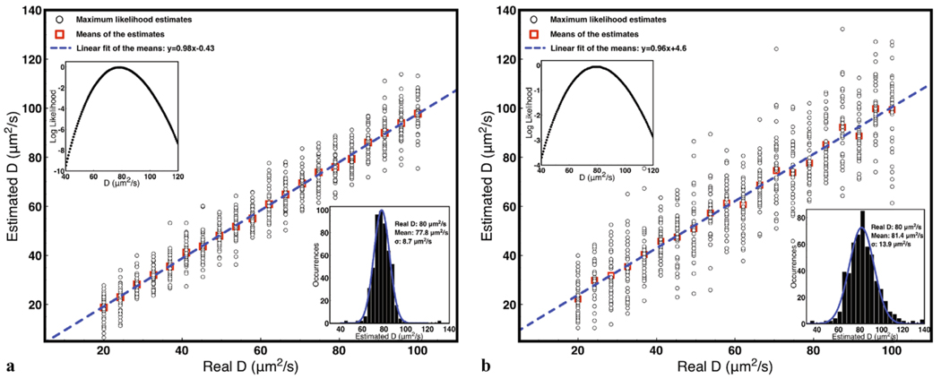
Maximum likelihood estimation of diffusion coefficients using the algorithm developed in Sect. 3. The parameters used in the simulation are K = 0.4, g · μ = 8000 s⁻¹, Δt_max = 76.8 µs. Only the first 150 ms of trapping data are used in the estimation. (a) In case of high signal-to-background ratio (SBR ≈ 280). (b) In case of low signal-to-background ratio (SBR ≈ 4.7). Each diffusion coefficient is estimated 40 times and plotted as black circles, averages of the 40 estimates are shown as red squares. Dashed blue lines are linear fits of the means, y = 0.98x − 0.43 in (a) and y = 0.96x + 4.6 in (b). Left inset: behavior of log likelihood vs. assumed D from single trapping runs (with assumed D = 80 µm²/s). Right inset: histograms of 500 estimates with assumed D = 80 µm²/s and Gaussian fits. The standard deviation of the estimated diffusion coefficients are 8.7 µm²/s in the high SBR case and 13.9 µm²/s in the low SBR case