Figure 3.
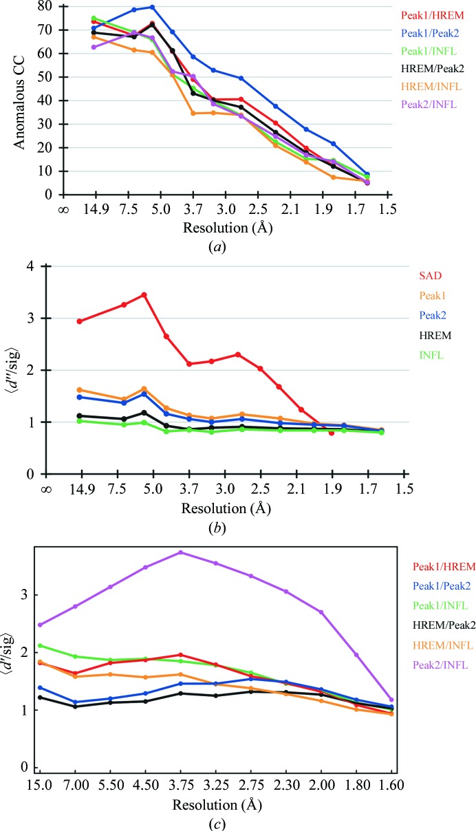
Anomalous and dispersive data statistics. (a) Anomalous correlation coefficient (CC) between the MAD data sets. HREM, high-energy remote; INFL, inflection point (data-collection wavelengths can be found in Table 1 ▶). The correlation coefficients do not depend on the (estimated) σ values. Data were truncated at 2.5 Å for heavy-atom substructure solution (where CC falls below 30% for all data sets). (b) Anomalous signal for the four bromine MAD data sets and the iodine SAD data set (red); pure noise would correspond to d′′/sig ≃ 0.798. Here, the cutoff for the MAD data sets cannot be determined easily. The iodine data set shows a strong anomalous signal (data collected at 1.5418 Å). Data were truncated at 2.0 Å for heavy-atom substructure solution for the iodine data set (where d′′/sig falls below 1.2). (c) Dispersive differences between the MAD data sets. HREM, high-energy remote; INFL, inflection point (data-collection wavelengths can be found in Table 1 ▶). Radiation damage could have caused the apparent differences in d′ values; because one wavelength was completed before the next wavelength was measured, systematic errors could be introduced that could also lead to an overestimation of the dispersive signal.

