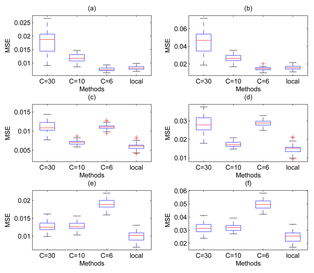
Figure 7.

Simulated MS data: Comparison of global and local thresholding schemes over the 2,000 – 15,000 m/z range ((a), (c) and (e)) and the 2,000 – 5,000 m/z range ((b), (d) and (f)). In each plot, the first three boxplots refer to Coombes et al. method with C = 30, C = 10, and C = 6, respectively, and the last boxplot refers to our method. Plots in the upper row, (a) and (b), are for the case of a white noise error with constant variance, plots in the middle row, (c) and (d), for the case of a white noise error and monotonic decreasing variance. Plots in the bottom row, (e) and (f), refer to the case of an autoregressive error with monotonic decreasing variance. Results have been obtained using universal thresholds for the white noise error cases and the level-dependent threshold of Johnstone and Silverman for the case of correlated errors.