Figure 1.

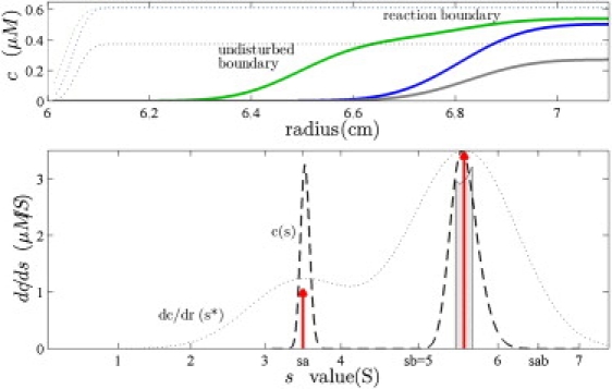
(Top) Concentration profiles calculated from Lamm PDE solutions for species A (3.5 S, green) reversibly interacting with B (5 S, blue) to form transient complexes AB (6.5 S, gray), sedimenting at 60,000 rpm. Initially, c_Atot(r,t = 0) = c_Btot(r,t = 0) = K_D, and shown are c_k(r,t) at 5 min (dotted) and t^∗ = 100 min (solid lines). (Bottom) Experimentally, from the measured total signal, c_Atot(r,t^∗) + c_Btot(r,t^∗) could be easily determined an apparent velocity distribution g^∗(s^∗) ∼ dc/dr (dotted line), or the diffusion-deconvoluted sedimentation coefficient distribution c(s) (23) (dashed line). The asymptotic boundary $d\widehat{c}/ds$ from GJT is shown as a light gray bar, and the predictions from EPT are shown as red arrows (scaled to represent the relative signal amplitudes, assuming equal signal increments).