Joint Prior Models of Neighboring Objects for 3D Image Segmentation

Abstract

This paper presents a novel method for 3D image segmentation, where a Bayesian formulation, based on joint prior knowledge of multiple objects, along with information derived from the input image, is employed. Our method is motivated by the observation that neighboring structures have consistent locations and shapes that provide configurations and context that aid in segmentation. In contrast to the work presented earlier in [1], we define a Maximum A Posteriori (MAP) estimation model using the joint prior information of the multiple objects to realize image segmentation, which allows multiple objects with clearer boundaries to be reference objects to provide constraints in the segmentation of difficult objects. To achieve this, muiltiple signed distance functions are employed as representations of the objects in the image. We introduce a representation for the joint density function of the neighboring objects, and define joint probability distribution over the variations of objects contained in a set of training images. By estimating the MAP shapes of the objects, we formulate the joint shape prior models in terms of level set functions. We found the algorithm to be robust to noise and able to handle multidimensional data. Furthermore, it avoids the need for point correspondences during the training phase. Results and validation from various experiments on 2D/3D medical images are demonstrated.

I. Introduction

Image segmentation remains an important and challenging task due to poor image contrast, noise, and missing or diffuse boundaries. To address these problems, Snakes or Active Contour Models (ACM) (Kass et al. (1987)) [2] have been widely used for segmenting non-rigid objects in a wide range of applications, where an initial contour is deformed towards the boundary of the object to be detected by minimizing an energy functional. These methods maybe sensitive to the starting position and may “leak” through the boundary of the object if the edge feature is not salient enough.

In more sophisticated deformable models, the incorporation of more specific prior information into deformable models has received a large amount of attention. Cootes et al. [3] find corresponding points across a set of training images and construct a statistical model of shape variation from the point positions. The best match of the model to the image is found by searching over the model parameters. Staib and Duncan [4] incorporate global shape information into the segmentation process by using an elliptic Fourier decomposition of the boundary and placing a Gaussian prior on the Fourier coefficients. Zeng et al. [5] develop a coupled surfaces algorithm to segment the cortex by using a thickness prior constraint. Leventon et al. [6] extend Caselles' [7] geodesic active contours by incorporating shape information into the evolution process.

Our work is also a prior-information-based approach to image segmentation. As an extention of the neighbor-constraint deformable model presented earlier in [1], our work shares the observation that neighboring structures have consistent locations and shapes that provide configurations and context that aid in segmentation. In contrast to the work presented in [1], the MAP segmentation framework that we present in this paper is based on a joint prior information of the multiple objects in the image (instead of using the conditional local neighbor prior information). The objects with clearer boundaries in the image can be used as reference objects to provide constraints in the segmentation of difficult objects. Our work also shares the common aspects with a number of coupled active contour models [1][5][8], where multiple level set functions are employed as the representations of the multiple objects within the image. By using this level-sets based numerical algorithm, several objects can be segmented simultaneously.

The strength of our approach is the incorporation of joint prior information of multiple objects into image segmentation to improve the segmentation results as well as reduce the complexity of the segmentation process by providing prior constraints from multiple neighboring objects. Our model is based on a MAP framework using the joint prior information of neighboring objects within the image. We introduce a representation for the joint density function of the neighbor objects and define the corresponding probability distributions. Formulating the segmentation as a MAP estimation of the shapes of the objects and modeling in terms of level set functions, we compute the associated Euler-Lagrange equations. The contours evolve while attempting to adhere to the neighbor prior information and the image gray level information.

II. Description of the Model

A. MAP Framework with Joint Prior Information Of Multiple Objects

As presented in our previous work in [1], probabilistic formulations are powerful approaches to deformable models. Deformable models can be fit to the image data by finding the model shape parameters that maximize the posterior probability. Consider an image I that has M shapes of interest; a MAP framework can be used to realize image segmentation combining joint prior information of the neighboring objects and image information:

$$\begin{array}{cc}\hfill {\widehat{S}}_i& ={\arg \max }_{S_i}p(S_1,S_2,\dots ,S_i,\dots ,S_M\mid I)\hfill \\ \hfill & =\arg \max S_{i}p(I\mid S_1,S_2,\dots ,S_M)p(S_1,S_2,\dots ,S_M)i=1,2,\dots ,M\hfill \end{array}$$ (1)

where S₁, S₂, …, S_M are the evolving surfaces of all the shapes of interest.

p(I|S₁, S₂, …, S_M) is the probability of producing an image I given S₁, S₂, …, S_M. In 3D, assuming gray level homogeneity within each object, we use the following imaging model [9]:

$$\begin{array}{cc}\hfill & p(I\mid S_1,S_2,\dots ,S_M)\hfill \\ \hfill & =\prod _{i=1}^M\{\prod _{(x,y,z)\mathit{inside}\left(S_i\right)}\exp [-\frac{{\left(I(x,y,z)c_{1i}\right)}^2}{2{\sigma }_{1i}^2}]\phantom{\}}\hfill \\ \hfill & \phantom{\{}\cdot \prod _{(x,y,z)\mathit{outside}\left(S_i\right),\mathit{inside}\left({\Omega }_i\right)}\exp [-\frac{{(I(x,y,z)-c_{2i})}^2}{2{\sigma }_{2i}^2}]\}\hfill \end{array}$$ (2)

where c_1i and σ_1i are the average and variance of I inside S_i, c_2i and σ_2i are the average and variance of I outside S_i but also inside a certain domain Ω_i that contains S_i.

p(S₁, S₂, …, S_M) is the joint density function of all the M objects. It contains the neighbor prior information such as the relative position and shape among the objects. In many cases, objects to be detected have one or more neighboring structures with known or clearer boundaries in the image. These known or easily segmented objects can be used as reference objects to provide constraints in the segmentation of those difficult objects. Assume S₁ = ξ₁, S₂ = ξ₂, …, S_l = ξ_l (1 ≤ l < M) are the known shapes in the image, S_l+1, S_l+2, …, S_M are the difficult shapes to be segmented. Then the MAP framework in equation (1) can be written in this form:

$$\begin{array}{cc}\hfill & {\widehat{S}}_i=\hfill \\ \hfill & {\arg \max }_{S_i}[p(I\mid S_1={\xi }_1,S_2={\xi }_2,\dots ,S_l={\xi }_l,S_{l+1},\dots ,S_M)\hfill \\ \hfill & \cdot p(S_1={\xi }_1,S_2={\xi }_2,\dots ,S_l={\xi }_l,S_{l+1},\dots ,S_M)]i=l+1,l+2,\dots ,M,1\le l<M\hfill \end{array}$$ (3)

B. Joint Prior Model Of Multiple Objects

To build a model for the joint prior of the neighboring objects, we choose level sets as the representation of the shapes [1][6][8], and then define the joint probability density function p(S₁, S₂, …, S_M) in equation (1).

Consider a training set of n aligned images {I₁, I₂, …, I_n}, with M objects or structures of interest in each image. The surfaces of each of the Mn shapes in the training set are embedded as the zero level set of Mn separate higher dimensional level sets with negative distances inside and positive distances outside the object, as shown below:

$$T=\left[\begin{array}{cccc}\hfill {\Psi }_{11}\hfill & \hfill {\Psi }_{12}\hfill & \hfill \dots \hfill & \hfill {\Psi }_{1n}\hfill \\ \hfill {\Psi }_{21}\hfill & \hfill {\Psi }_{22}\hfill & \hfill \dots \hfill & \hfill {\Psi }_{2n}\hfill \\ \hfill \hfill & \hfill \dots \hfill & \hfill \hfill & \hfill \hfill \\ \hfill {\Psi }_{M1}\hfill & \hfill {\Psi }_{M2}\hfill & \hfill \dots \hfill & \hfill {\Psi }_{Mn}\hfill \end{array}\right]$$ (4)

Using the technique developed in [6], each of the Ψ_ij(i = 1, 2, …, M; j = 1, 2, …n) is placed as a column vector with N^d elements, where d is the number of spatial dimensions and N^d is the number of samples of each level set function. We can use vector ${\chi }_j={[{\Psi }_{1j}^T,{\Psi }_{2j}^T,\dots ,{\Psi }_{Mj}^T]}^T$ as the representation of the M objects of interest in image I_j. Thus, the corresponding training set is {χ₁, χ₂, …, χ_n}. Our goal is to build a joint model of the multiple objects over the distribution of the level sets vector χ.

Following the lead of [6][8], the mean and variance of the level sets vector χ can be computed using Principal Component Analysis (PCA). The mean level sets vector, $\stackrel{‒}{\chi }$, is calculated using

$$\stackrel{‒}{\chi }=\frac{1}{n}\sum _{j=1}^n{\chi }_j$$ (5)

For each level sets vector χ_j in the training set we calculate its deviation from the mean, dχ_j, where

$$d{\chi }_j={\chi }_j-\stackrel{‒}{\chi },j=1,2,\dots ,n$$ (6)

Then each such deviation is placed as a column vector in a MN^d × n dimensional matrix Q. Using Singular Value Decomposition (SVD), Q = UΣV^T. U is a matrix whose column vectors represent the set of orthogonal modes of joint variation of the M objects and Σ is a diagonal matrix of corresponding singular values. An estimate of the joint level sets of the M objects χ can be represented by k principal components and a k dimensional vector of coefficients α (where k < n)[3]:

$$\tilde{\chi }=\stackrel{‒}{\chi }+U_k\alpha$$ (7)

To write equation (7) in the level sets form, we have:

$$\widetilde{\left[\begin{array}{c}\hfill {\Psi }_1\hfill \\ \hfill {\Psi }_2\hfill \\ \hfill ⋮\hfill \\ \hfill {\Psi }_M\hfill \end{array}\right]}=\stackrel{‒}{\left[\begin{array}{c}\hfill {\Psi }_1\hfill \\ \hfill {\Psi }_2\hfill \\ \hfill \cdots \hfill \\ \hfill {\Psi }_M\hfill \end{array}\right]}+U_k\alpha$$ (8)

Under the assumption of a Gaussian distribution of joint level sets represented by α, the joint probability density function of neighboring objects, p(S₁, S₂, …, S_M), can be approximated by:

$$p\left(\alpha \right)=\frac{1}{\sqrt{{\left(2\pi \right)}^k\mid {\Sigma }_k\mid }}\exp [-\frac{1}{2}{\alpha }^T{\Sigma }_k^{-1}\alpha ]$$ (9)

Figure 1 shows a few of the 16 MR cardiac training images used to define the level set based shape model of the endocardial boundary of the left and right ventricles. Before computing and combining the level sets of these training shapes, the curves were rigidly aligned. By using PCA of the joint level sets of the two structures, we can build a model of the joint shapes of left and right ventricles. Figure 2 illustrates zero level sets corresponding to the mean and three primary modes of variance of the distribution of the two ventricles jointly.

Fig. 1.

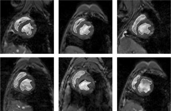
Outlines of left and right ventricles in 6 out of 16 2D MR cardiac training images gated and at a fixed point in the cardiac cycle.

Fig. 2.

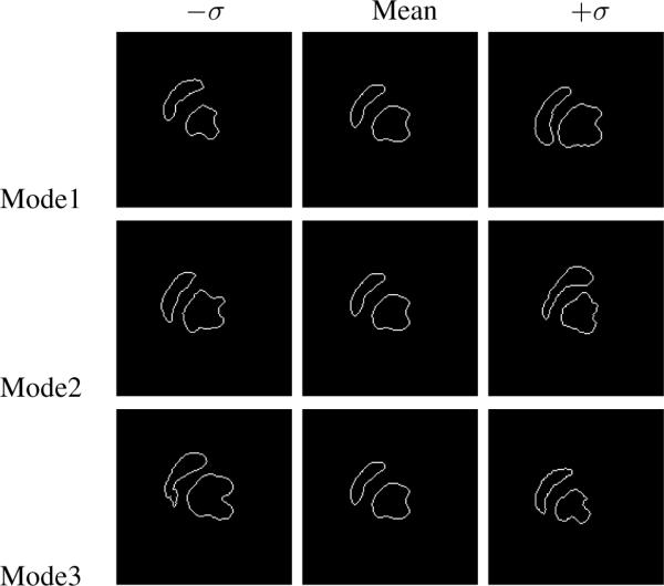
The three primary modes of variance of the left and right ventricles.

We also show a 3D training set of two rigidly aligned subcortical structures: the left amydala and left hippocampus in Figure 3. Figure 4 shows the three primary modes of variance of the left amydala and left hippocampus. Note that the zero level sets of the mean joint level sets and primary modes appear to be reasonable representative shapes of the classes of objects being learned. This shows that our joint prior model of multiple objects successfully incorporates the neighbor prior information such as the relative position and shape among the objects and unifies them under one framework.

Fig. 3.

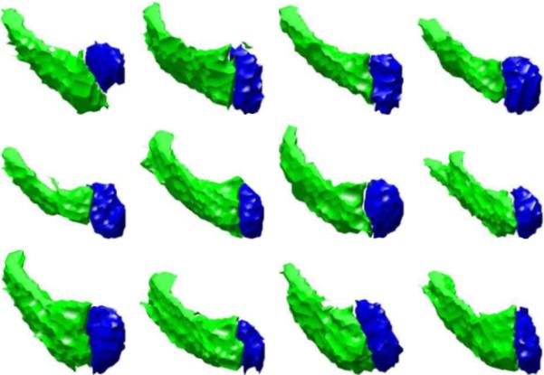
Zero level sets of two post-aligned subcortical structures-left amydala and left hippocampus in 12 3D MR training images.

Fig. 4.

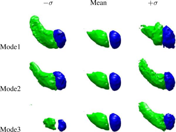
The three primary modes of variance of the left amydala and left hippocampus.

In our active contour model, we also add some regularizing terms [1]: a general smoothness Gibbs prior for the region boundaries p_B(S₁, S₂, …, S_M) and a model for the size of the region p_A(S₁, S₂, … S_M).

$$p_B(S_1,S_2,\dots ,S_M)=\prod _{i=1}^M{e}^{-{\mu }_i{\oint }_{S_i}ds}$$ (10)

$$p_A(S_1,S_2,\dots ,S_M)=\prod _{i=1}^M{e}^{-{\nu }_i{A}_i^c}$$ (11)

where A_i is the size of the region of shape i, c is a constant and μ_i and ν_i are scalar factors. Here we assume the boundary smoothness and the region size of all the objects are independent. Thus, the joint prior probability p(S₁, S₂, … S_M) can be approximated by a product of the following probabilities:

$$\begin{array}{cc}\hfill p(S_1,S_2,\dots ,S_m)=& p\left(\alpha \right)\cdot p_B(S_1,S_2,\dots ,S_M)\hfill \\ \hfill & \cdot p_A(S_1,S_2,\dots ,S_M)\hfill \end{array}$$ (12)

Therefore, equation (1) can be approximated by:

$$\begin{array}{cc}\hfill & p(S_1,S_2,\dots ,S_M\mid I)\hfill \\ \hfill & \propto \prod _{i=1}^M\{\prod _{(x,y,z)\mathit{inside}\left(S_i\right)}\exp [-\frac{{(I(x,y,z)-c_{1i})}^2}{2{\sigma }_{1i}^2}]\hfill \\ \hfill & \cdot \prod _{(x,y,z)\mathit{outside}\left(S_i\right),\mathit{inside}\left({\Omega }_i\right)}\exp [-\frac{{(I(x,y,z)-c_{2i})}^2}{2{\sigma }_{2i}^2}]\}\hfill \\ \hfill & \cdot \prod _{i=1}^M{e}^{-{\mu }_i{\oint }_{S_i}ds}\prod _{i=1}^M{e}^{-{\nu }_i{A}_i^c}\hfill \\ \hfill & \cdot \frac{1}{\sqrt{{\left(2\pi \right)}^k\mid {\Sigma }_k\mid }}\exp [-\frac{1}{2}{\alpha }^T{\Sigma }_k^{-1}\alpha ]\hfill \end{array}$$ (13)

Since:

$$\begin{array}{cc}\hfill {\widehat{S}}_i& ={\arg \max }_{S_i}p(S_1,S_2,\dots ,S_i,\dots ,S_M\mid I)\hfill \\ \hfill & ={\arg \min }_{S_i}[-{\log }_{e}p(S_1,S_2,\dots ,S_i,\dots ,S_M\mid I)]i=1,2,\dots ,M\hfill \end{array}$$ (14)

Let

$$\begin{array}{cc}\hfill & E=-\ln p(S_1,S_2,\dots ,S_i,\dots ,S_M\mid I)\hfill \\ \hfill & \propto {\Sigma }_{i=1}^M\{{\lambda }_{1i}\cdot {\int }_{(x,y,z)\mathit{inside}\left(S_i\right)}{\mid I(x,y,z)-c_{1i}\mid }^{2}dxdydz\hfill \\ \hfill & +{\lambda }_{2i}\cdot {\int }_{(x,y,z)\mathit{outside}\left(S_i\right),\mathit{inside}\left({\Omega }_i\right)}{\mid I(x,y,z)-c_{2i}\mid }^{2}dxdydz\}\hfill \\ \hfill & +{\Sigma }_{i=1}^M{\mu }_i{\oint }_{S_i}ds+{\Sigma }_{i=1}^M{\nu }_i{A}_i^c+{\omega }_i{\alpha }^T{\Sigma }_k^{-1}\alpha \hfill \end{array}$$ (15)

Given the first l objects in the image, the MAP estimation of the other shapes of interest in equation (3), ${\widehat{S}}_i(i=l+1,l+2,\dots ,M)$, is also the minimizer of the above energy functional E. This minimization problem can be formulated and solved using the level set method and we can realize the segmentation of multiple objects simultaneously.

C. Level Set Formulation of the Model

In the level set method, S_i is the zero level set of a higher dimensional level set ψ_i corresponding to the i th object being segmented, i.e., S_i = {(x, y, z)|ψ_i(x, y, z) = 0}. The evolution of surface S_i is given by the zero-level surface at time t of the function ψ_i(t, x, y, z). We define ψ_i to be positive outside S_i and negative inside S_i. Each of the M objects being segmented in the image has its own S_i and ψ_i.

For the level set formulation of our model, we replace S_i with ψ_i in the energy functional in equation (15) using regularized versions of the Heaviside function H and the Dirac function δ, denoted by H_ε and δ_ε [9] (described below):

$$\begin{array}{cc}\hfill & E(c_{1i},c_{2i},{\psi }_i\mid i=l+1,l+2,\dots M)\hfill \\ \hfill & ={\Sigma }_{i=l+1}^M\{{\mu }_i{\int }_{\Omega }{\delta }_{\epsilon }\left({\psi }_i(x,y,z)\right)\mid \nabla {\psi }_i(x,y,z)\mid dxdydz\hfill \\ \hfill & +{\nu }_i{\int }_{\Omega }(1-H_{\epsilon }\left({\psi }_i(x,y,z)\right))dxdydz\hfill \\ \hfill & +{\lambda }_{1i}{\int }_{\Omega }{\mid I(x,y,z)-c_{1i}\mid }^2(1-H_{\epsilon }\left({\psi }_i(x,y,z)\right))dxdydz\hfill \\ \hfill & +{\lambda }_{2i}{\int }_{{\Omega }_i}{\mid I(x,y,z)-c_{2i}\mid }^2{H}_{\epsilon }\left({\psi }_i(x,y,z)\right)dxdydz\}\hfill \\ \hfill & +{\omega }_i[{(G\left({\psi }_1\right)-\stackrel{‒}{{\psi }_1})}^T,{(G\left({\psi }_2\right)-\stackrel{‒}{{\psi }_2})}^T,\dots ,{(G\left({\psi }_M\right)-\stackrel{‒}{{\psi }_M})}^T]\hfill \\ \hfill & \cdot U_k{\Sigma }_k^{-1}{U}_k^T\hfill \\ \hfill & \cdot {[{(G\left({\psi }_1\right)-\stackrel{‒}{{\psi }_1})}^T,{(G\left({\psi }_2\right)-\stackrel{‒}{{\psi }_2})}^T,\dots ,{(G\left({\psi }_M\right)-\stackrel{‒}{{\psi }_M})}^T]}^T\hfill \end{array}$$ (16)

where Ω denotes the image domain. G(·) is an operator to generate the vector representation(as shown in section II-B) of a matrix by column scanning. g(·) is the inverse operator of G(·). To compute the associated Euler-Lagrange equation for each unknown level set function ψ_i, we assume that the M − l difficult objects are related to the l easy neighbor objects independently, keep c_1i and c_2i fixed, and minimize E with respect to ψ_i (i = l + 1, l + 2, …M) respectively. Parameterizing the descent direction by artificial time t ≥ 0, the evolution equation in ψ_i(t, x, y, z) is:

$$\begin{array}{cc}\hfill \frac{\partial {\psi }_i}{\partial t}& ={\delta }_{\epsilon }\left({\psi }_i\right)[{\mu }_i\cdot \mathit{div}\left[\frac{\nabla {\psi }_i}{\mid \nabla {\psi }_i\mid }\right]+{\nu }_i\hfill \\ \hfill & +{\lambda }_{1i}{\mid I-c_{1i}\mid }^2-{\lambda }_{2i}{\mid I-c_{2i}\mid }^2]\hfill \\ \hfill & -{\omega }_i\cdot g\left[U_{ki}{\Sigma }_k^{-1}{U}_{ki}^T(G\left({\psi }_i\right)-{\stackrel{‒}{\psi }}_i)\right]\hfill \\ \hfill & -{\omega }_i\cdot g\left[U_{ki}{\Sigma }_k^{-1}\sum _{j=1}^l\left[U_{kj}^T(G\left({\psi }_i\right)-{\stackrel{‒}{\psi }}_j)\right]\right]\hfill \\ \hfill & i=l+1,l+2,\dots M\hfill \end{array}$$ (17)

where U_ki is the k_th part of the matrix U_k respectively, i.e., ${\left[U_k\right]}^T=[U_{k1}^T,U_{k2}^T,\dots ,U_{kM}^T]$. Each U_ki has the same size.

D. Evolving the Surface

We approximate H_ε and δ_ε as follows [9]: $H_{\epsilon }\left(z\right)=\frac{1}{2}[1+\frac{2}{\pi }\arctan \left(\frac{z}{\epsilon }\right)]$, ${\delta }_{\epsilon }\left(z\right)=\frac{\epsilon }{\pi ({\epsilon }^2+z^2)}$. c_1i and c_2i are defined by: $c_{1i}\left({\psi }_i\right)=\frac{{\int }_{\Omega }I(x,y,z)\cdot (1-H\left({\psi }_i(x,y,z)\right))dxdydz}{{\int }_{\Omega }(1-H\left({\psi }_i(x,y,z)\right))dxdydz}$, $c_{2i}\left({\psi }_i\right)=\frac{{\int }_{{\Omega }_i}I(x,y,z)\cdot H\left({\psi }_i(x,y,z)\right)dxdydz}{{\int }_{{\Omega }_i}H\left({\psi }_i(x,y,z)\right)dxdydz}$.

Given the surfaces ψ_i(i = 1, 2, …M) at time t, we seek to compute the evolution steps that bring all the zero level set curves to the correct final segmentation based on the joint prior information of the objects and image information. We first set up p(α) from the training set using PCA. At each stage of the algorithm, we recompute the constants $c_{1i}\left({\psi }_i^t\right)$ and $c_{2i}\left({\psi }_i^t\right)$ and update ${\psi }_i^{t+1}$. This is repeated until convergence.

To simplify the complexity of the segmentation system, we generally choose the parameters in our experiments as follows: λ_1i = λ_2i = λ_i, μ_i = 0.00005·255², ν_i = 0 [9]. This leaves us only two free parameters (ω_i and λ_i) to balance the influence of two terms, the image data term and the neighbor prior term for each object. The tradeoff between neighbor prior and image information depends on the strength of the neighbor prior and the image quality for a given application. We set these parameters empirically for particular segmentation tasks, given the general image quality and the neighbor prior information.

III. Applications to Medical Imagery

We have used our model on various medical images, with at least two different types of shapes, at least one of which can be regarded as the reference object. All the tested images are not in their training sets. The variations captured by the principal components in level set based distribution model (U_k)in this paper are based on rigid alignment of the training data.

We first consider a 2D cardiac image with two structures of interest, the left and right ventricles. The training set consists 16 images like those in Figure 1. In Figure 5 top, we show the segmentation of the left and right ventricles using only image information, by which the curves cannot lock onto the shapes of the objects. In Figure 5 bottom, we show the results obtained using our model, where the right ventricle is the reference object. The curves are able to converge on the desired boundaries even though some parts of the boundaries are too blurred to be detected using only gray level information. Both of the segmentations converged in a couple of minutes on a 2.00GHz Intel XEON CPU.

Fig. 5.

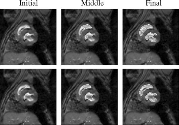
Three steps in the segmentation of 2 shapes in a 2D cardiac MR image without (top) and with (bottom) neighbor prior (λ_i = ω_i = 0.5, i = 1, 2).

We then consider a 2D MR brain image with eight subcortical structures of different intensities and with blurred boundaries. Figure 6 shows a few of the zero level sets of post-aligned eight subcortical structures from 12 2D MR training images. Figure 7 top shows a few steps of the segmentation using only gray level information. Only the lower (posterior) portions of the lateral ventricles can be segmented perfectly since they have clearer boundaries. Figure 7 bottom shows the results of using our joint shape prior model, where the ventricles are the reference objects for all the other objects. Segmenting all eight subcortical structures took approximately several minutes.

Fig. 6.

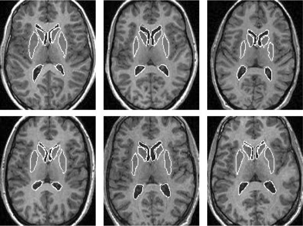
Outlines of 8 sub-cortical structures in 6 out of 12 MR training images.

Fig. 7.

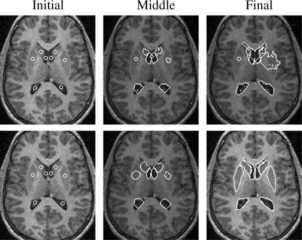
Segmentation of 8 sub-cortical structures (the lateral ventricles (λ_i = 0.8, ω_i = 0.2), heads of the caudate nucleus (λ_i = 0.3, ω_i = 0.7), and putamina (λ_i = 0.2, ω_i = 0.8)) in a MR brain image without prior information (top) and with joint shape prior (bottom).

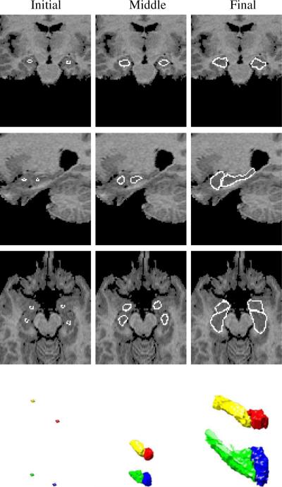
We also test our method using 3D medical images. Figure 8 shows a few steps in the segmentation of the left and right amygdalae and hippocampi in a MR brain image. Segmentating the four structures can be very tough without using prior information since all of them have very poorly defined boundaries. After using our neighbor constraint joint prior model, as shown in Figure 8, the four structures can be clearly segmented, where we choose the amygdalae as the references since they have relative smaller variances of the shapes. Segmenting these 3D images (with size 172 × 148 × 124) took approximately a couple of hours.

Fig. 8.

Initial, middle, and final steps in the segmentation of left and right amygdalae and hippocampi (λ_i = 0.1, ω_i = 0.9, i = 1, 2, 3, 4.) in a 3D MR brain image. Three orthogonal slices (coronal, sagittal, and axial) and the 3D surfaces are shown for each step. The training set consists of 12 MR images.

To validate the segmentation results, we test our model on 12 different images for each of the above 3 cases respectively, the tested images are not in their training sets. We then compute the undirected average distances of pixels between the boundaries of the computed segmentation A (N_A points) and the boundaries of the manual segmentation B: H(A, B) = max(h(A, B), h(B, A)), $h(A,B)=\frac{1}{N_A}{\Sigma }_{a\in A}^{}{\min }_{b\in B}\Vert a-b\Vert$. For our experiments, the mean distances show improvement in all the 3 cases comparing with/without the joint shape prior as shown in Table 1. Virtually all the boundary points obtained using our model lie within one or two voxels of the manual segmentation.

TABLE I.

Distance between the computed and manual boundaries

(Unit:[pixel])	Cardiac	2D brain	3D brain
no prior	9.2	8.3	5.8
with prior	1.6	2.0	2.2

We also test the robustness of our algorithm to noise. We add Gaussian noise to the MR image in Figure 7 (the mean intensities of white/gray matters: 70/48), then segment it. Figure 9 shows the segmentation results with Gaussian noise of standard deviation of 20 (left), 30 (middle) and 40 (right). In Figure 10, we show the segmentation errors of the lower portion of the left lateral ventricle in three cases: with no prior, with shape prior, and with joint neighbor prior. As the variance of the noise goes up, the error for no prior increases rapidly since the structure is too noisy to be detected using only gray level information. However, for the methods with shape prior and with joint neighbor prior, the errors are much lower and are locked in a very small range even when the variance of the noise is very large. Note that our joint neighbor joint prior model achieves the smallest error among all the cases.

Fig. 9.

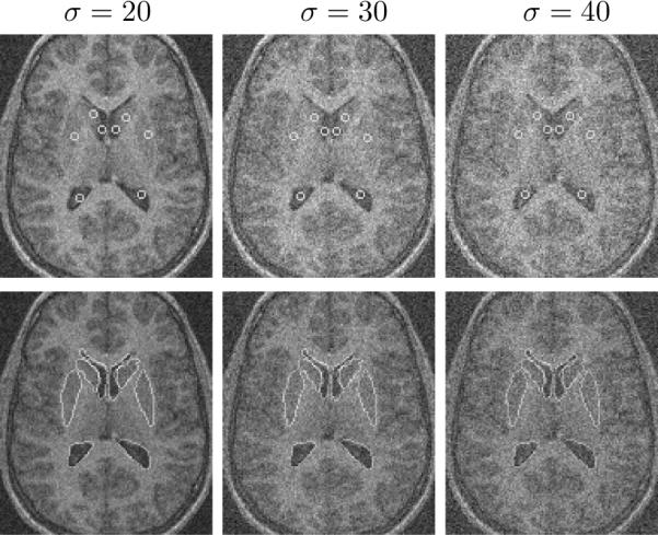
Initial and final steps in the segmentation of 8 sub-cortical structures in a MR brain image with Gaussian noise of σ = 20 (left), σ = 30 (middle), and 40 (right).

Fig. 10.

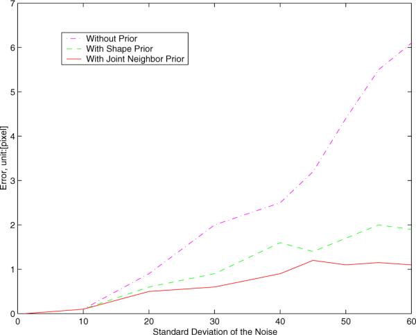
Segmentation errors (unit:[pixel]) with different variances of Gaussian noise.

In our work, we have focused on balancing the weights of the image data (λ_i) and neighbor prior (ω_i) with all the other parameters fixed. For all the applications presented in the paper, the weights of the image data and prior information can be varied by around 30% with the corresponding segmentation errors changing by no more than 5%. Thus, our method is not sensitive to the balance of the weights.

IV. Conclusion

A new model for automated segmentation of images containing multiple objects by incorporating neighbor prior information in the segmentation process has been presented. We wanted to capture the constraining information that neighboring objects provided and use it for segmentation. We define a MAP estimation framework using the prior information provided by multiple neighboring objects to segment several objects simultaneously. We introduce a representation for the joint density function of the neighbor objects, and define joint probability distributions over the variations of the neighboring positions and shapes in a set of training images. We estimate the MAP shapes of the objects using evolving level sets based on the associated Euler-Lagrange equations. The contours evolve both according to the neighbor prior information and the image gray level information. Multiple objects in an image can be automatically detected simultaneously.

References

- [1].Yang J, Staib L, Duncan J. Neighbor-Constrained Segmentation with 3D Deformable Models. IPMI. 2003:198–209. doi: 10.1007/978-3-540-45087-0_17. [DOI] [PubMed] [Google Scholar]
- [2].Kass M, Witkin A, Terzopoulos D. Snakes: Active contour models. Int'l Journal on Computer Vision. 1987;1:321–331. [Google Scholar]
- [3].Cootes TF, Hill A, Taylor CJ, Haslam J. Use of active shape models for locating structures in medical images. Image and Vision Computing. 1994 July;12(6):355–365. [Google Scholar]
- [4].Staib L, Duncan J. Boundary finding with parametrically deformable models. PAMI. 1992;14(11):1061–1075. [Google Scholar]
- [5].Zeng X, Staib LH, Schultz RT, Duncan JS. Volumetric Layer Segmentation Using Coupled Surfaces Propagation. IEEE Conf. on Comp. Vision and Patt. Recog. 1998 [Google Scholar]
- [6].Leventon M, Grimson E, Faugeras O. Statistical shape influence in geodesic active contours. IEEE Conf. on Comp. Vision and Patt. Recog. 2000;1:316–323. [Google Scholar]
- [7].Caselles V, Kimmel R, Sapiro G. Geodesic active contours. Int. J. Comput. Vis. 1997;22(1):61–79. [Google Scholar]
- [8].Tsai A, Wells W, Tempany C, Grimson E, Willsky A. Coupled Multi-shape Model and Mutral Information for Medical Image Segmentation. IPMI. 2003:185–197. doi: 10.1007/978-3-540-45087-0_16. [DOI] [PubMed] [Google Scholar]
- [9].Chan T, Vese L. Active Contours Without Edges. IEEE Transactions on Image Processing. 2001;10(2):266–277. doi: 10.1109/83.902291. [DOI] [PubMed] [Google Scholar]