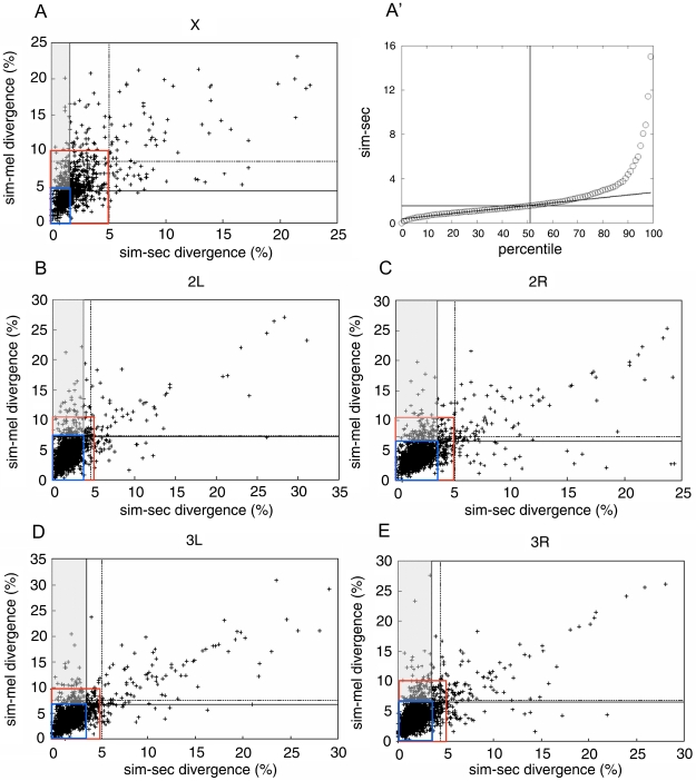
Figure 2. Patterns of divergence along chromosomes and two screening methods.

A, B, C, D and E) Each graph corresponds to a chromosome or chromosome arm (X, 2L, 2R, 3L and 3R), where the genes are ordered from the least divergent to the most divergent in sim-sec (abscissa) and sim-mel (ordinate). The horizontal and vertical dashed lines delimit the averages plus one standard deviation of the divergence between sim-sec (horizontal) and sim-mel (vertical). The upper left quadrants delimit genes found by the method of averages and standard deviations. Note that the divergences of most genes in all 5 graphs are clustered in a quadrant that can be roughly delimited between the abscissa values of 0%–5% and ordinate values 0%–10% (red rectangles). In this quadrant, the genes have a good fit with a linear distribution (P<0.0001). To better delimit the quadrant in which the divergence is linear in each chromosome, the data was divided in percentiles of divergences of sim-sec, sim-mel and sec-mel. (A') exemplifies the percentiles of the X chromosome. Since each point in these curves represents one percentile, the percentage of genes that diverge linearly is equal to the number of points that can be transected by a straight line. Once this linear interval is defined, the values on the x and y axes become known and can be used to redefine the quadrant of linear divergences (inferior left quadrant in blue). The region where the genes in sim-sec vary the least and the genes in sim-mel vary the most is the adjacent upper quadrant to the left of the point where the horizontal and vertical lines cross (gray quadrant).