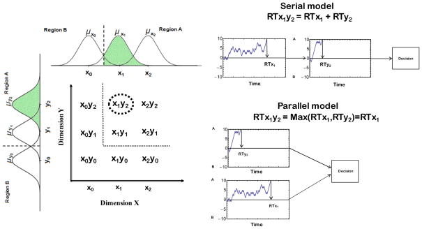
Figure 3.

Schematic illustration of the serial-exhaustive and parallel-exhaustive architectures, using stimulus x1y2 as an example. In the serial example, we assume that Dimension X is processed first. The value x1 lies near the decision boundary on Dimension X, so the random-walk process on that dimension tends to take a long time to complete. The value y2 lies far from the decision boundary on Dimension Y, so the random-walk process on that dimension tends to finish quickly. For the serial-exhaustive architecture, the two random walks operate sequentially, so the total decision time is just the sum of the two individual-dimension random-walk times. For the parallel-exhaustive architecture, the two random walks operate simultaneously, and processing is not completed until decisions have been made on both dimensions, so the total decision time is the maximum (i.e., slower) of the two individual-dimension random-walk times.