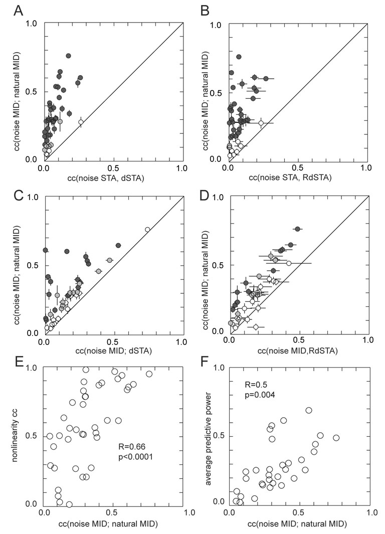
Figure 6. Correlation between spatiotemporal filters of the linear and LN models with noise and natural stimuli.

Similarity between two spatiotemporal filters is quantified by their correlation coefficient (c.c., or normalized dot product). For all cells, stimuli, and methods for estimating filters, the filter dimensionality was 16×16×3, 16 pixels horizontally, 16 pixels vertically, and 3 time lags. Panel A: c.c.’s between MID filters computed for noise and natural stimuli (y–axis) is plotted as a function of c.c.’s between the dSTA filter computed from natural stimuli and the STA filter computed from noise stimuli. Panel B is the same as A, except that the comparison on the x-axis is between the RdSTA filter computed from natural stimuli and the STA filter computed from noise stimuli. In panels C and D, the noise filter is computed as the MID in comparison to both the natural MID filter (y-axis) and either the dSTA filter (x-axis for panel C or the RdSTA filter (x-axis for panel D). Error bars show standard deviations. Solid line has a slope of one. In panels A–D, color indicates statistical significance of deviation from identical cc’s (white, p>0.05; gray, 0.01<p<0.05; black, p<0.01, t-test). Greater similarity between spatiotemporal MID filters under natural and noise stimulation is associated with greater similarity in the corresponding nonlinear gain functions (panel E, p<10⁻⁴, R=0.66) and greater average predictive power of natural MID for neural responses to a novel segment of natural scenes and of noise MID to responses for novel segment of noise (panel F, p=0.004, R=0.5).