Drug interaction: focusing on response surface models

Abstract

Anesthesiologists have been aware of the importance of optimal drug combination long ago and performed many investigations about the combined use of anesthetic agents. There are 3 classes of drug interaction: additive, synergistic, and antagonistic. These definitions of drug interaction suggest that a zero interaction model should exist to be used as a reference in classifying the interaction of drug combinations. The Loewe additivity has been used as a universal reference model for classifying drug interaction. Most anesthetic drugs follow the sigmoid E_max model (Hill equation); this model will be used for modeling response surface. Among lots of models for drug interaction in the anesthetic area, the Greco model, Machado model, Plummer model, Carter model, Minto model, Fidler model, and Kong model are adequate to be applied to the data of anesthetic drug interaction. A model with a single interaction parameter does not accept an inconsistency in the classes of drug interactions. To solve this problem, some researchers proposed parametric models which have a polynomial interaction function to capture synergy, additivity, and antagonism scattered all over the surface of drug combinations. Inference about truth must be based on an optimal approximating model. Akaike information criterion (AIC) is the most popular approach to choosing the best model among the aforementioned models. Whatever the good qualities of a chosen model, it is uncertain whether the chosen model is the best model. A more robust inference can be extracted from averaging several models that are considered relevant.

Introduction

In anesthesia, a synergistic effect of the combined treatments gives patients the following favorable outcomes: increasing the efficacy of the anesthetic effect, reducing doses while increasing or maintaining the same efficacy to avoid toxicity of anesthetic drugs, minimizing or slowing the development of drug resistance, and providing selective synergism against the target (or efficacy synergism) versus the host (or toxicity antagonism) [1]. Many such studies can be found in related literature [2-8].

There are 3 classes of drug interaction: additive interaction, in which the response of a drug combination is just what is expected from the dose-response relationships of drugs; synergistic interaction, in which the response is greater than expected; and antagonistic interaction, in which the response is less than expected. There is no uniform agreement on the terminology of drug interaction. Synonyms for what is termed additive interaction are zero, or null interaction, independence (Bliss), and indifference. Synonyms for synergistic interaction are positive or supra-additive interaction, potentiation, and augmentation. Synonyms for antagonistic interaction are negative, infra-additive or subadditive interaction, and negative synergy. These definitions of drug interaction suggest that a zero interaction model should exist to be used as a reference in classifying the interaction of drug combinations. A pharmacodynamic model of most anesthetic drugs is the sigmoid E_max model (Hill equation); let's discuss drug interactions and response surface focusing on this model.

Reference models for zero interaction

Because the classification of drug interactions is determined as a greater or less pharmacological effect of a two-drug combination than what would be predicted for zero interaction from the knowledge of the effects of each drug individually, its determination absolutely depends on the reference model of zero interaction. A review by Berenbaum [9] has listed 8 approaches, and another review by Greco et al. [10] categorized 13 approaches and methods for determining the class of drug interaction. To define the class of drug interactions, first, an adequate reference model of additive (or zero) interaction should be established as a universal standard reference. Historically, 3 zero interaction models are commonly used [9,10]: Bliss independence [11], Loewe additivity [12], and the median-effect method from the law of mass action [13].

Bliss independence

Bliss independence implies that 2 drugs do not pharmacologically or physiologically cooperate with each other for each drug behaves independently of the other [10]. The general equations of Bliss independence (Eq. (1)) and a specific one (Eq. (2)), which assumes that a sigmoid E_max relationship [14,15] is an appropriate pharmacodynamic model for each drug, are as follows:

In Eq. (1), fu₁, fu₂, and fu₁₂ are the fractions of response for drug 1, drug 2, and combination unaffected [16]. In Eq. (2), 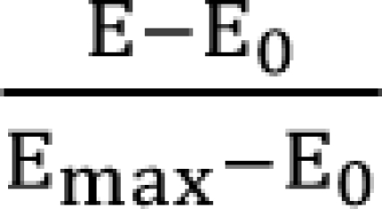is a fraction of the effect resulting from the mixture of d₁ and d₂; d₁ and d₂ are doses of each drug in the mixture that yield the effect E; ED_{50,1 or 2} is a dose of drugs to produce 50% of the maximal effect (E_max) for each drug acting alone; and γ₁ and γ₂ are Hill coefficients (slope of dose-response curve). When Eq. (1) and (2) are recast in terms of the fraction of effect affected (fa_{1 or 2}) (if 1 - fa exchanges fu in Eq. (1), because fa + fu = 1), then Eq. (3) and (4) are the results.

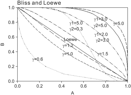
Eq. (3) is similar to the equation of probabilities of independent events [17]. The curvature of the Bliss independence line depends on the Hill coefficient of each drug (Fig. 1).

Fig. 1.

Normalized isoboles at 50% effect level, for the Bliss independence model, Eq. (2), for various values of γ₁ and γ₂, which are listed next to each corresponding curve. A single γ indicates that γ₁ = γ₂ = γ. When Hill coefficients are different (one larger than) 1.3 and the other less than 1.2), the isoboles are S-shaped and may cross the Loewe additivity diagonal line. The solid diagonal line is The Loewe additivity line (Eq. (5)). The isobole for zero interaction of a mutually nonexclusive model (Eq. (9)) is the same curve as that of the Bliss independence model with γ = 1.0.

Loewe additivity

Lines connecting points representing equi-effective dose combinations are termed isoboles (Fig. 1). They were introduced by Fraser [18,19], who claimed that, in using this device for evaluating the antagonism between the actions of physostigmine and atropine, "the results of the experiment will be rendered apparent by a mere glance at the diagram." Loewe extended this method to synergism [12,20]. Loewe used a straight line isobole for zero interaction when the combined drugs had similar mechanisms of action and similar dose-response relationship, and asserted that the isobole would be curved when combined drugs had different mechanisms of action and dissimilar dose-response relationship. Recently, Tallarida [21] supported Loewe's assertion. When a full agonist and a partial agonist have different maximum values, or when Hill coefficients (γ of sigmoid E_max model) of two full agonist drugs are different, each case has a varying potency ratio. For a full agonist and a partial agonist, the isobole of no interaction is no longer straight but curved [22]. For two full agonists with a varying potency, termed "heterodynamic" by Loewe [12], the application of dose equivalence leads to not just one, but to two nonlinear additive isoboles [21,23]. However, Berenbaum [9] maintained that a straight-line isobole is appropriate for a zero interactive combination, for it is not derived from the knowledge of the shapes of the dose-response curves or of their mechanisms of action, and he concluded that it is valid irrespective of the shapes of these curves, similar or dissimilar, and also, irrespective of their mechanisms of action. Although the shape of the isobole for Loewe additivity remains to be further studied, a straight line of additivity is commonly employed to distinguish synergistic and antagonistic from additive interactions. Although there are many reasons to prefer the Berenbaum method, the most predominate reason to use it may be because of easy calculations.

The general equation of the Loewe additivity (Eq. (5)) and a specific form (Eq. (6)), which assumes that a sigmoid E_max relationship is appropriate for each drug, is defined as

where d₁ and d₂ are doses of each drug in the mixture that yield an effect, E, while D_{1 or 2} is the dose of each drug to produce the same effect of E when given alone. The term 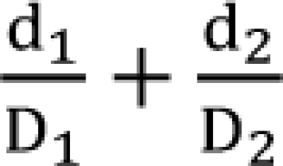is called the interaction index at the combination dose (d₁, d₂). The dose (D₁, or D₂) for each single drug producing the same effect of E is expressed as

If the interaction index at (d₁, d₂) is equal to, less than, or greater than 1, the combination dose is asserted to be additive, synergistic, or antagonistic, respectively.

Median-effect method from the law of mass action

The median-effect principle (Eq. (7)) was originated by Chou [24,25]. The median-effect equation describes dose-response relationship in the simplest terms, which is given by

where d is the dose of a drug; f_a is the fraction affected by d; f_u is the fraction unaffected by d (i.e., f_u = 1 - f_a, and f_a / f_u = odds ratio); D_m is the median effect dose (e.g. EC₅₀, or ED₅₀); and m is the slope coefficient of dose-response curve. When m is greater than 1, the dose-response curve becomes S-shaped, so m is equivalent to the Hill coefficient of sigmoid E_max equation.

Chou and Talalay [16] extended the median-effect equation for a single drug to multiple drugs. Thus, for a two-drug interaction, they got the same equation of combination index (CI) (Eq. (8)) as that of the interaction index by Berenbaum [26]. This equation is based on the assumption that two drugs bind the same receptors and are mutually exclusive. This gives

where d₁ and d₂ are doses of each drug in the mixture that yield an effect, f_a, while D_{1 or 2} is the dose of each drug to produce the same effect of f_a when given alone. D_{m,1 or 2} is the median effect dose of drug 1 or drug 2, and m_{1 or 2} is the slope coefficient of dose-response curve of drug 1 or drug 2. In the view of interaction, CI < 1, = 1, and > 1 indicate synergy, additivity, and antagonism, respectively.

If it is assumed that two drugs do not share receptors, do not interfere with each other, and are mutually nonexclusive, the resulting equation (Eq. (9)) should include a third term, the product of the first two terms, thus,

As shown in Fig. 1, the isobole of CI for the mutually nonexclusive model is concave upward, and is identical to that of the Bliss independence model (Eq. (4)) in which the Hill coefficient (γ) of sigmoid E_max model is 1. Therefore, this model under-estimates synergistic effects.

Because partially exclusive or partially nonexclusive cases may exist, and the equation with the third term may underestimate synergistic effects, Chou [1] claimed that the equation without the third term should be used as the "base equation" and that mutual non-exclusivity should be used as a contributing factor for the intrinsic synergistic effect under the assumption of mutual exclusivity. To be consistent with the classic isobologram and its equation (interaction index of Berenbaum), he decided that mutually exclusive assumption will be used for the analysis of drug interaction.

The Bliss independence and Loewe additivity models are the two most cited reference models for determining drug interaction [9,10,27,28]. According to Berenbaum, only when the dose-response relationship of each drug follows an exponential decline with the dose, the two models result in the same equation and are consistent with each other [10]. When dose-response curves are steeper than the exponential model, Bliss independence will result in Loewe antagonism; whereas, when dose-response curves are less steep than the exponential model, Bliss independence will result in Loewe synergism (Fig. 1). Greco et al. [10] revealed that they prefer Loewe additivity to Bliss independence for the lack of synergism or antagonism. When curves are steep (γ > 2), the Bliss independence criterion may overestimate synergism, whereas the Loewe additivity model can overemphasize antagonism. That is to say, a class of drug interaction is dependent on a reference model because a given effect seems to be either synergistic with the Loewe additivity or antagonistic with the Bliss independence. However, the use of both models is not practical because one of the two models could be more plausible than the other [27]. Goldoni and Johansson [27] said that although the Loewe additivity model is slightly more plausible and is preferred in toxicology, it could be incorrect under certain conditions.

The interpretation of an assessment of drug interactions by the Loewe additivity reference model is free of mechanistic restrictions and implications. It is possible to determine that the combination of two or more inhibitors is more effective than their individual use by means of isobolographic analysis, even when no information about their mechanism of action is available [29]. Accordingly, the Loewe additivity reference model is consistent with the graphical isobologram approach [29]. The sigmoidicity of a dose-effect curve greatly magnifies the differences among the different methods or theories (Fig. 1). Thus, the main controversies in drug combination analysis in the past century can be readily resolved [1]. Drug additivity is substantiated under the Loewe additivity model but not the Bliss independence model [30]. Therefore, the Loewe additivity model is a universal reference model for classifying drug interaction.

Response surface

There have been several methods for evaluating drug inter-action: diagonal array [17], isoboles [9,17,31], isobolar surface for three-drug combination [17], interaction index [9,17], and response surface [10]. Isobolographic analysis and interaction index method are not universally applicable, and they rely on the level of effect; one isobole relates only to a single effect, and one interaction index does only to a single dose pair. Therefore, separate analyses should be conducted at numerous levels (ED₅, ED₂₅, ED₅₀, ED₇₅, etc.) in order to classify all possible interactions. To depict the entire set of levels of effect (from ED₁ to ED₉₉), one may build all the isoboles in three dimensions, thus, creating a surface of isoboles, the so-called response surface. It illustrates the drug effect (Z axis) versus two-drug doses (X and Y axes) [10] and presents an entire drug interaction at all dose pairs.

Over the last decade, drug interaction studies have been increasingly evaluated on the basis of a response surface model. The approaches to choosing a response surface model are empirical or functional [32]. Many examples of response surface methods employed a single interaction parameter to catch synergy, additivity, or antagonism [33-37]. These models are sound if only synergy, additivity, or antagonism exists throughout the entire surface; they are incompetent to describe the interspersion of regional synergy or regional antagonism in different areas of drug combinations [38].

Isoboles are not necessarily consistent or similar because they may cross the additivity line so that some combinations with a specific effect are synergistic, and others antagonistic. Berenbaum maintained that the conclusion as to whether a combination has a specific class of drug interaction applies to that combination but not to untested combinations [9]. A model with a single interaction parameter never reflects an inconsistency in the patterns of drug interactions. To solve this problem, some researchers proposed a few parametric models with a polynomial interaction function for two drugs [38-40]. The interaction functions capture synergy, additivity, and antagonism scattering all over the surface of drug combinations.

Response surface models with a single interaction parameter

Greco model [34]

Assuming the dose-response relationships for two drugs follow the sigmoid E_max, the formula of this model is:

The interaction parameter is α, which catches the magnitude of synergy, additivity, or antagonism. Because , , the first two terms on the right-hand expression of Eq. (11) are equivalent to Eq. (5). Thus, Eq. (12) defines interaction index for two-drug combination.

Therefore, when α > 0, the interaction index is less than 1, Loewe synergism is indicated; when α < 0, interaction index is greater than one, Loewe antagonism is indicated; and when α = 0, Loewe additivity is indicated. The larger positive α is, the smaller the interaction index and the stronger the synergy.

Machado model

Machado and Robinson [35] reviewed a set of interaction models which were provided by Hewlett [41], and they recommended the ensuing model, which was in effect considered by Plackett and Hewlett [42]:

Like the parameter α in the model of Greco et al. [34]. the interaction parameter is η. When 0 < η < 1, Loewe synergism is indicated; when 1 < η < ∞, Loewe antagonism is indicated; and when η = 1, Loewe additivity is indicated. The smaller the value of η with 0 < η < 1, the more synergistic is the interaction.

Plummer model

Plummer and Short [36] used a model, Eq. (14), for identifying and quantifying departures from additivity. Their model is a generalization of a model with a fixed relative potency derived by Finney [33], and it allows relative potency to vary. Their model is:

where Y is the transformed effect (logit), and ρ is a relative potency of drug 2 versus drug 1 given by

D_{1 or 2} is the dose of each drug to produce the same effect of E when given alone. The Newton-Raphson method is used to find D'₂ in the Plummer model. For this model, the plots of Y versus log (d) for two drugs should be linear but need not be parallel. This model contains five parameters (β₀, β₁, β₂, β₃, and β₄). When you set d₂ = 0 or d₁ = 0 for Eq. (14), you will get , 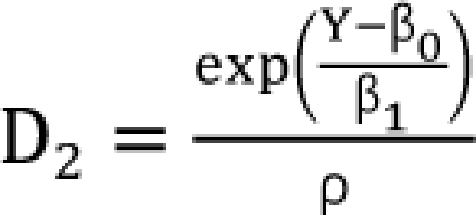which are the doses of drug 1 and drug 2 producing the effect E. You can rearrange Eq. (14) to be

Therefore, β₄ is the interaction parameter which captures synergism (β₄ > 0), additivity (β₄ = 0), and antagonism (β₄ < 0). The larger positive is β₄, the smaller the interaction index, and the stronger the synergy.

Carter model

The multivariate linear logistic model [43] is very popular in the analysis of clinical trial data when the response variables are binary or quantal. Carter et al. [37] and Gennings et al. [44] used the logistic model for an analysis of drug interactions involving continuous data points. They rearranged the general form of the logistic model and used the following equation:

Setting d₁ = d₂ = 0, you will get the dose (D₁, and D₂) of each drug 1 or drug 2 alone eliciting an effect E: , . After moving β₀ to the left side of Eq. (17), and then dividing both sides of the equation with , you will obtain the interaction index:

The denominator must be positive. β₁₂ is the interaction parameter which captures synergism (β₁₂ > 0), additivity (β₁₂ = 0), or antagonism (β₁₂ < 0).

There are many other parametric response surface models with a single interaction parameter; they can be applied to the common data. Hewlett [41] provided a general framework for deriving many specific, potentially-useful, multivariate interaction models. All response surface models using a single interaction parameter are inappropriate in the situation when synergism, additivity, and antagonism intersperse over the entire range of doses.

Response surface models with an interaction function

Minto model

Minto et al. [39] employed the concept of normalizing drug concentration to potency. They thought that any ratio (θ) of the two drugs acts like a new drug, and a fixed ratio of the two drugs (a new drug) has its own sigmoid E_max curve. The sigmoid E_max model for a single drug is extended to a model that takes each ratio of two drugs as a drug in its own right.

I will express the concentrations of drugs V and R as [V] and [R]. Each drug must be normalized to its potency, C₅₀, and the following forms are obtained.

U_V and U_R are units of potency, and the normalized concentrations of drugs V and R. A set of new drugs, each having a unique unit ratio (θ) of U_V and U_R, is defined in a set of terms of θ. The term of θ is defined as

When only drug V exists, θ is 0; when only drug R exists, θ is 1. The new drug concentration is simply U_V + U_R. These terms can be combined with the sigmoid E_max equation:

where the drug concentration is U_V + U_R, then γ(θ) is the sigmoidicity of the concentration-response curve at a specific ratio (θ); U₅₀(θ) is the number of units of potency associated with 50% of the maximum effect at a specific ratio θ; and E_max(θ) is the maximum drug effect at a specific ratio θ. The term U₅₀(θ) is the potency of drug combination at a specific ratio θ. Because one 50% of maximum effect is 1 unit of potency, when only drug V (θ = 0) or drug R (θ = 1) is present, the number of units associated with one 50% drug effect, U₅₀(0) or U₅₀(1), must be one.

Minto et al. chose the fourth-order polynomial function (f(θ)) to allow the interspersion of patterns of drug interactions all over the drug combinations.

The forms of f(θ) are E_max(θ), U₅₀(θ), and γ(θ). Coefficients β_x are model parameters that are estimated by the data. The two terms, β₀ and β₁ in E_max(θ), U₅₀(θ), or γ(θ), are replaced by other terms already defined.

If U₅₀(θ) is 1 for all values of θ, the interaction will be additive. If U₅₀(θ) is less than 1 for all values of θ, this amplifies the term 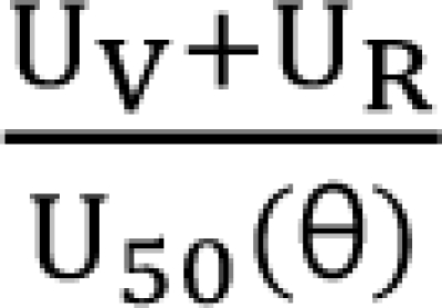in Eq. (21). This will create a synergistic effect. If U₅₀(θ) is greater than 1 for all values of θ, this lessen the term in Eq. (21). This will create an antagonistic effect. This model can be used in investigating the drug interaction when the maximum effects of drugs V and R are not identical.

The functions of parameters for the Minto model are unable to interpret the classes of drug interactions which mix themselves over the whole response surface. The contours of interaction indices will make the interpretation easy by a mere glance at the plot. The equation for the interaction index is as follows:

The values of C_50,V, C_50,R, γ_V, and γ_R will be yielded after a given data is fitted to this model. The specific effect E is produced by the combination of [V] and [R].

Fidler model

Fidler et al. [40] criticized the Minto model for weakness in quantitative analysis of the degree of interaction. Therefore, they developed the flexible interaction model [40], which can provide parameters to help clinicians immediately determine the interaction surface shape, interaction type, maximum interaction point, and interaction curve shape. The Fidler model meets Minto's criteria for an ideal pharmacodynamic interaction model [39] and is similar to the Finney model in that both models have the interaction term of square root [33].

A general form is

The term α indicates the type of interaction. Positive values show synergy; negative ones show antagonism. The term f defines changes in an isobole of the response surface for a given level of drug effect. A functional form of the term f inspired by the gamma probability distribution gives

In this function, θ is identical to θ in Minto model and is given 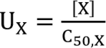, 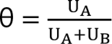. The m term is the symmetry parameter of the potency ratio θ, where the maximum interaction occurs. The interaction scope parameter w specifies the uniformity of the interaction across various drug ratios. The parameters γ(θ) and E_max(θ) are given as functions of potency fraction:

The linear functions of the potency ratio, [γ_Aθ + γ_B(1-θ)], and [E_max,Aθ+E_max,B(1-θ) are simple estimates for γ(θ) and E_max(θ). The parameters β and ζ influence the type of change in the linear estimates of γ(θ) and E_max(θ). Positive values of β and ζ indicate an increase in γ(θ) and E_max(θ); negative indicates a decrease in them; and 0 means no change from the line of estimates of γ(θ) and E_max(θ). The terms, β·f(m_β,w_β,θ) and ζ·f(m_β,w_β,θ), are restricted to be greater than -1 to keep each function positive. The parameters m_β and m_ζ are the symmetry parameters of the respective changes, where the maximum changes in γ(θ) and E_max(θ) occur; the parameters w_β and w_ζ are the line shape parameters around m_β and m_ζ, and are greater than 0.

When the Hill slopes of two drugs are different [21], both the Minto and Fidler models deviate from the classic additive interaction surface as given by Berenbaum [9]. Fidler et al. [40] demonstrated that by assuming a simple linear change in the Hill slope as a function of potency fraction, the predicted differences between a classical additive interaction state and the additive interaction state of the Minto or Fidler model are less than experiment error and can be considered negligible.

In practical considerations, a direct transformation of the α term (% contribution of α ) expresses % change of the 50% effect when compared with each drug in combination acting alone. Another feature is for the Fidler model to predict the concentration ratio of two drugs at the most effective points. In an asymmetric case, the best ratio is C_50,V × m : C_50,R × (1 - m); in a symmetric case, the best ratio is C_50,V : C_50,R.

Kong model

Kong and Lee [38] used Chou and Talalay's [16] median effect equation (Eq. (8)) as a dose-response curve for a single agent. In Eq. (8), when f(a) replaces E, and logarithm is applied to the modified equation, the median effect equation has the form . It is assumed that the logit-transformed response follows a linear function of log (d) for each of two drugs when acting independently. The dose-response curve denotes . The model proposed by Kong and Lee has a square root term and the relative potency. So, it can be regarded as a generalization of Finney's model [33] and the model derived by Plummer and Short [36]. To construct a generalized model, including the nonparallel dose-response curves of two drugs, a varying relative potency should be allowed. When the two drugs have the nonparallel dose-response curves, or different slopes, each drug combination ([V], [R]) on the z-isobole shares the same relative potency ρ(z), and its equivalent amount dose is [V] + ρ(z) [R] in terms of drug V, or ρ(z)^-1 [V] + [R] in terms of drug R. That is, the combination doses on different isoboles may have different relative potencies. The form of ρ(z) is derived as

[V]_iso and [R]_iso are the respective single drug doses of drug V and drug R, and each of them creates the effect z. To describe the interspersion of interaction modes, Kong and Lee use the following form as an interaction function:

where f is an interaction polynomial function of [V] and [R] with parameters γ₁ and γ₂ capturing the varying relative potency ρ and the coefficients δ's. The above polynomial function is substituted for the interaction parameter (β₄) of the Plummer model, and the following equation is given as

Like the interaction index of the Plummer model, the interaction index of the Kong model could be derived as the following form:

When the polynomial function is greater than, equal to, or less than 0, the interaction index is less than, equal to, or greater than 1, and the resulting interaction is synergistic, additive, or antagonistic, respectively.

Data analysis

The analyses of the following data were performed using the 7 methods reviewed here. The aim of the study was to investigate the combinations of vecuronium and rocuronium to have synergistic interaction. Left phrenic nerve-hemidiaphragms of 48 male Sprague-Dawley rats (150-250 g in weight) were mounted in Krebs solution. Supramaximal electrical stimulation (0.2 ms, rectangular) of 50 Hz for 1.9 s was applied to the phrenic nerve, and the evoked tetanic contractions were measured with a force transducer. Each preparation was exposed to one of four vecuronium concentrations (0.0, 1.5, 2.5, 3.0 µM), or one of four rocuronium concentrations (0.0, 3.0, 4.5, 5.5 µM). Subsequently the adequate amount of rocuronium to a vecuronium bath or vecuronium to a rocuronium bath was cumulatively added until an 80-90% increase of tetanic fade was reached.

In this data set, E₀'s of two drugs are 0, and E_max's are 1 (or 100%). For interaction parameter and interaction index of the Greco, and Machado models, the values of Hill slope and potency of each drug acting alone were calculated (vecuronium: 6.5125, 2.98 µM, rocuronium: 7.8975, 5.34 µM, respectively) and then substituted for ED₅₀'s and γ's of the two models. Interaction indices of the Berenbaum method (Eq. (5)) were directly calculated using the sigmoid E_max equation substituted with the above calculated values. Plummer model (Eq. (14)) and Carter Model (Eq. (17)) were fitted with the data by using Tablecurve3D®.

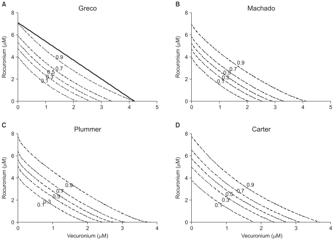
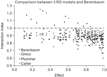
The iso-effective contours (Fig. 2) and the plot of interaction indices of actual data points (Fig. 3) were drawn. All the isoboles of the 4 models are upward concave and consistently indicate synergistic interaction (Fig. 2). The interaction index of the Machado model cannot be calculated due to the limitation of the model. Table 1 shows the results of five interaction analysis methods. Four models, except for the Berenbaum method, consistently show interaction indices of less than 1, which mean synergistic interaction (Table 1 and Fig. 3). In Fig. 3, the Berenbaum method reveals that the interaction indices are less than 1 at the high effect region and are greater than 1 at the low effect region. According to the Berenbaum method, combinations of the two drugs have all types of interaction. Therefore, the response surface models with a single interaction parameter are inadequate to analyze the data which has complicated scatter of different types of drug interactions (Fig. 3 and 4, Panel A).

Fig. 2.

The Greco model (A), the Machado model (B), the Plummer model (C), and the Carter model (D) show isoboles of the response surface. The abscissa is a concentration of vecuronium (µM) and the ordinate, that of rocuronium (µM). The numbers in the plots are the fractional increase of tetanic fade. The thick, solid line in panel A is shown as an example of the Loewe additivity line at a 0.9 effect. If all the Loewe additivity lines would be drawn, these would reveal that the isoboles are upward concave. Therefore, it is concluded that interactions between vecuronium and rocuronium are consistently synergistic.

Fig. 3.

The plot of interaction indices of actual data points was drawn. The interaction index of the Machado model cannot be calculated due to the limitation of the model. Four models, except for the Berenbaum method, consistently have interaction indices of less than 1, which means synergistic interaction. The Berenbaum method reveals that most interaction indices are less than 1 at a high effect region, and are greater than 1 at a low effect region. According to the Berenbaum method, combinations of the two drugs have all types of interaction. Therefore, the response surface models with a single interaction parameter are inadequate in analyzing data which has a complicated scatter of different types of drug interactions.

Table 1.

Five Methods for Detecting Drug Interactions in Combined Vecuronium and Rocuronium

Estimated value of Berenbaum is mean of IaI's. IaI indicates interaction index by Berenbaum method, Sy indicates synergy, CI indicates confidence interval.

Fig. 4.

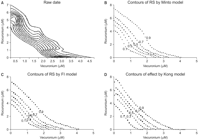
This figure shows isoboles of the response surface derived from raw data (A), Minto model (B), Fidler model (C), and Kong model (D). The isoboles of raw data (A) are rendered via the Renka I (nonparametric algorithm) procedure. The abscissa is a concentration of vecuronium (µM) and the ordinate, that of rocuronium (µM). The numbers in the plots are the fractional increase of tetanic fade. If the Loewe additivity line would be drawn, this would reveal what type of drug interaction the isobole has.

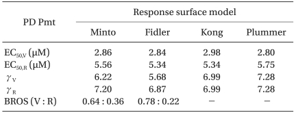
Next, three aforementioned flexible response surface models with an interaction function were fitted to the same data using Tablecurve3D®, and the parameters, the response surfaces, isoboles, and contours of the interaction index of each model were determined, and plots were made for seeking the differences of their results (Fig. 4 and 5). The functions for the parameters U₅₀(θ) and γ(θ) of the Minto model were calculated and illustrated (Fig. 6). The full model (10 parameters) for the Minto model was analyzed; the Fidler model (9 parameters) was analyzed when w = 1; and the Kong model (8 parameters) was analyzed when the relative potency ratio was constant. The isobole plot of raw data is rendered via Renka I (nonparametric algorithm) procedure, and it is shown in Fig. 4, panel A. Pharmacodynamic parameters of response surface models are listed at Table 2. The values are different depending on the model. In the Kong and Plummer models, because relative potency ratio is constant, the Hill slopes of each model are identical.

Fig. 5.

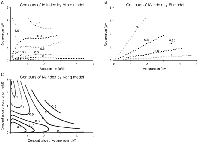
The contours of the interaction index calculated based on the Minto model (A), Fidler model (B), and Kong model (C) are plotted. The value "1.0" in the contour plot of the interaction indices represents additivity; the values less than 1.0 represent synergistic interaction; and the ones more than 1.0 represent antagonistic interaction. Chou and Hayball proposed that an interaction index from 0.9 to 1.1 is designated as being additive. Based on the Minto and Fidler models, the interactions of the two drugs are synergistic and additive. By the Kong model, the interactions of the two drugs are synergistic, additive, and antagonistic. The interspersion of the interaction indices on the entire surface is relatively different among three models. The abscissa is a concentration of vecuronium (µM) and the ordinate, that of rocuronium (µM).

Fig. 6.

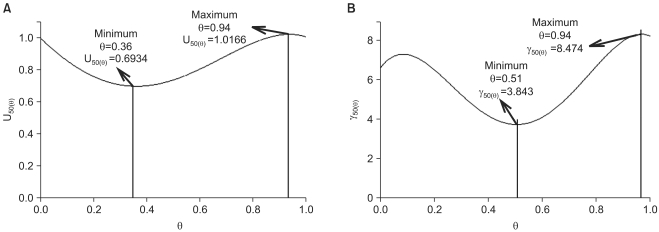
The functions for the parameters U₅₀(θ), and γ(θ) for the two drug interaction show a synergistic interaction (U₅₀(θ)=0.6934) at θ=0.36, which is the ratio of the potency unit of 0.64 : 0.36, vecuronium : rocuronium (A), and varying steepness depending on the unique ratio of two drugs (B).

Table 2.

Pharmacodynamic Parameters of RS Models

BROS (V : R): best ratio of synergy (vecuronium : rocuronium), EC_50,V and EC_50,R: median effect of vecuronium and rocuronium, respectively, γ_V and γ_R : Hill slope of vecuronium and rocuronium, PD Pmt: pharmacodynamic parameter, RS: response surface, Kong and Plummer: assume that relative potency ratio is constant (or the dose-effect curves are parallel).

The isobole plots of the Minto model, Fidler model, and Kong model were relatively similar to the isobole plot of raw data. Minto et al. determined the pattern of drug interaction based on the functions of E_max, U₅₀(θ), and γ(θ), especially the value of U₅₀(θ) (Fig. 6). The isobole plot of the Minto model is shown in Fig. 4, panel B. In this article, with the equation of the interaction index, the contour plot of the interaction index (Fig. 5, panel A) can be illustrated and help to make the quantitative evaluation. Chou and Hayball [45] proposed that an interaction index from 0.9 to 1.1 is designated as being additive. In the Minto model, the lower extreme effect region has greater synergistic interaction. Chou [13] said that for anticancer or antiviral agents, synergy at high effect levels (fa > 0.8) is more relevant to therapy than at low effect levels (fa < 0.2). On the contrary, in the anesthetic area, synergy at low effect levels may be more crucial than at high levels because the residual effects of anesthetic agents could threaten the safety of patients.

In the Fidler model, the pattern of drug interaction is determined based on contour of iso-effective combinations, contour of interaction index, a direct transformation of the α term (% contribution of α on a 50% effect), and the best ratio for synergistic effect. The isobologram (Fig. 4, panel C) shows the deepest upward concavity around the combination of the unit ratio of 0.78 : 0.22, vecuronium : rocuronium (Table 2). The interaction indices range from 1 to 0.78. According to Chou and Hayball [45], the contour plot of interaction index (Fig. 5, panel B) reveals synergistic interaction, except for the area in which the combination of two drugs has a higher concentration of rocuronium than of vecuronium. A direct transformation of the α term (% contribution of α on a 50% effect) is 5% in this data set. In other words, the interaction of vecuronium and rocuronium requires 95% of the additive drug combination to produce the 50% effect at the most effect ratio. The minimum interaction index (0.78) is in about a 99% effective zone. The way in which to make this discrepancy has not been determined within the course of this research.

In the Kong model, it is assumed that relative potency is constant (that is, two drug dose-effect curves are parallel) like the analysis of the Plummer model. The shape of isobole in this model is most similar to that in the raw data among seven models (Fig. 4, panel A and D). The pattern of drug interaction is determined based on isobole plot, contour of interaction index, and polynomial function (not seen here). According to the Chou and Hayball [45], the isobologram (Fig. 4, panel D) shows synergistic, additive, and antagonistic interactions, and the interaction indices range from more than 1 to less than 0.6 (Fig. 5, panel C). The extreme effect regions get greater synergistic interaction.

The distribution of patterns of drug interaction depends on a response surface model. Which model best approximates the information in data should be decided using the model selection.

Model selection

The information scientists want to reveal is in the observed data. It has been expressed as a model. Making valid inferences from scientific data depends on a model of the information in the data [46]. For selecting the best model, it is assumed that there are data and a priori set of models and that statistical inference is to be model-based.

Researchers should conceive many models (i.e., multiple working hypotheses) and at the same time, cope with how to choose among the possibilities. The approaches to model selection use classical hypothesis testing [47], the Akaike information criterion (AIC) [48], the Bayesian information criterion (BIC) [49], and cross validation, etc. [46]. Generally, hypothesis testing is a very poor basis for model selection [48], especially, tests between models that are not nested [46]. In cross validation, the data are divided into two partitions, the first partition is used for model fitting; and the second one is used for model validation. A new partition is continuously selected, and this whole process is repeated hundreds or thousands of times. This method may be an alternative method for model selection but is time-consuming.

The target models of AIC and BIC are different [50]. The target model of AIC is specific to the sample size; it is the best model to minimize the estimated Kullback-Leibler information loss [51,52] when models are used to approximate the full reality (or truth). This target model depends on the change of sample size. Even the priori set of models may change when the sample size changes greatly. In contrast with AIC, the derivative assumption of BIC is that there is a true model in a model set. A true model is one that generates the data, independent of data size. The target model of BIC is the true model. The goal of model selection is to obtain a perfect model so that no information is lost in fitting data to a model of the information in data. It is impossible to achieve this ideal purpose because models are only approximations. However, AIC helps us choose the best model, which loses as little information as possible and allows the efficient and objective filtration of information from noise [46].

The principle of parsimony is that model selection is a bias versus variance trade-off. A parsimonious model must be as simple as possible in terms of variables and model structure. Inference from a model with too few variables may be biased, and inference from a model with too many variables may not be precise and can result in spurious conclusions. Parsimony lies between underfitting and overfitting [46]. For linear models, such as multiple regression, a minimum of 10 to 15 observations (or events) per predictor variable will generally allow good estimates [53-56]. Many researchers do not notice the problem of overfitting in regression-type modeling. Overfitting results in overly-optimistic findings that do not present in the real population and will not reproduce in a future data set. Although overfitting is not a bad beginning to seek a good model, spurious conclusions generated by overfitted model may lead doctors the wrong way in clinical decision-making.

In this article, 7 models are introduced, and the last 3 models have several nested submodels. A model should be selected to best fit a dose-effect data set using AIC, not hypothesis testing.

Summary

In anesthetic practice, anesthesiologists administer multiple drugs to patients simultaneously. They have been long aware of the importance of drug interaction and have performed many investigations for the efficient combination of anesthetic agents. The study of drug interaction is aiming at choosing the optimal drug combination.

Determining what pattern of drug interaction is acting is dependent on a reference model [10]. Although further study should be continued, Loewe additivity is a universal reference model for the classification of drug interaction. The reference model has been established, and then, many analytic models for drug interaction were proposed to be validated for their performances.

A lot of models have prevailed. In the anesthetic area, models with a single interaction parameter or flexible models with an interaction function are adequate to be applied to analyzing the data of anesthetic drug interaction. Due to detecting the best approximating model among the aforementioned models, AIC is the most popular approach for choosing the best model.

However good a chosen model may be, it never finds out the truth which generates the data set, and, of course, it is uncertain whether a chosen model is the best model for approximating information in the data. Instead of making an inference from only a chosen model estimated as the best, a more robust inference can be extracted from averaging several models that are considered relevant. This procedure is called multimodel inference [57], and this concept needs further study.

References

- 1.Chou TC. Theoretical basis, experimental design, and computerized simulation of synergism and antagonism in drug combination studies. Pharmacol Rev. 2006;58:621–681. doi: 10.1124/pr.58.3.10. [DOI] [PubMed] [Google Scholar]
- 2.Hendrickx JF, Eger EI, 2nd, Sonner JM, Shafer SL. Is synergy the rule? A review of anesthetic interactions producing hypnosis and immobility. Anesth Analg. 2008;107:494–506. doi: 10.1213/ane.0b013e31817b859e. [DOI] [PubMed] [Google Scholar]
- 3.Johnson KB, Syroid ND, Gupta DK, Manyam SC, Pace NL, Lapierre CD, et al. An evaluation of remifentanil-sevoflurane response surface models in patients emerging from anesthesia: model improvement using effect-site sevoflurane concentrations. Anesth Analg. 2009 doi: 10.1213/ANE.0b013e3181afe31c. [Epub ahead of print] [DOI] [PMC free article] [PubMed] [Google Scholar]
- 4.Syroid ND, Johnson KB, Pace NL, Westenskow DR, Tyler D, Bruhschwein F, et al. Response surface model predictions of emergence and response to pain in the recovery room: an evaluation of patients emerging from an isoflurane and fentanyl anesthetic. Anesth Analg. 2009 doi: 10.1213/ane.0b013e3181b11289. [Epub ahead of print] [DOI] [PMC free article] [PubMed] [Google Scholar]
- 5.Schumacher PM, Dossche J, Mortier EP, Luginbuehl M, Bouillon TW, Struys MM. Response surface modeling of the interaction between propofol and sevoflurane. Anesthesiology. 2009;111:790–804. doi: 10.1097/ALN.0b013e3181b799ef. [DOI] [PubMed] [Google Scholar]
- 6.Naguib M, Abdulatif M. Isobolographic and dose-response analysis of the interaction between pipecuronium and vecuronium. Br J Anaesth. 1993;71:556–560. doi: 10.1093/bja/71.4.556. [DOI] [PubMed] [Google Scholar]
- 7.Redai I, Richards KM, England AJ, Feldman SA. Interaction of decamethonium with hexamethonium or vecuronium in the rat: an isobolographic analysis. Anesth Analg. 1995;81:768–772. doi: 10.1097/00000539-199510000-00019. [DOI] [PubMed] [Google Scholar]
- 8.Paul M, Kindler CH, Fokt RM, Dipp NC, Yost CS. Isobolographic analysis of non-depolarising muscle relaxant interactions at their receptor site. Eur J Pharmacol. 2002;438:35–43. doi: 10.1016/s0014-2999(02)01271-2. [DOI] [PubMed] [Google Scholar]
- 9.Berenbaum MC. What is synergy? Pharmacol Rev. 1989;41:93–141. [PubMed] [Google Scholar]
- 10.Greco WR, Bravo G, Parsons JC. The search for synergy: a critical review from a response surface perspective. Pharmacol Rev. 1995;47:331–385. [PubMed] [Google Scholar]
- 11.Bliss CI. The toxicity of poisons applied jointly. Ann Appl Biol. 1939;26:585–615. [Google Scholar]
- 12.Loewe S. The problem of synergism and antagonism of combined drugs. Arzneimittelforschung. 1953;3:285–290. [PubMed] [Google Scholar]
- 13.Chou TC. Drug combination studies and their synergy quantification using the chou-talalay method. Cancer Res. 2010;70:440–446. doi: 10.1158/0008-5472.CAN-09-1947. [DOI] [PubMed] [Google Scholar]
- 14.Hill AV. The possible effects of the aggregation of the molecules of haemoglobin on its dissociation curves. J Physiol (Lond) 1910;40:iv–vii. [Google Scholar]
- 15.Sheiner LB, Stanski DR, Vozeh S, Miller RD, Ham J. Simultaneous modeling of pharmacokinetics and pharmacodynamics: application to d-tubocurarine. Clin Pharmacol Ther. 1979;25:358–371. doi: 10.1002/cpt1979253358. [DOI] [PubMed] [Google Scholar]
- 16.Chou TC, Talalay P. Quantitative analysis of dose-effect relationships: the combined effects of multiple drugs or enzyme inhibitors. Adv Enzyme Regul. 1984;22:27–55. doi: 10.1016/0065-2571(84)90007-4. [DOI] [PubMed] [Google Scholar]
- 17.Berenbaum MC. Criteria for analyzing interactions between biologically active agents. Adv Cancer Res. 1981;35:269–335. doi: 10.1016/s0065-230x(08)60912-4. [DOI] [PubMed] [Google Scholar]
- 18.Fraser TR. An experimental research on the antagonism between the actions of physostigma and atropia. Proc R Soc Edingburgh. 1870-1;7:506–511. [Google Scholar]
- 19.Fraser TR. The antagonism between the actions of active substances. Br Med J. 1872;2:485–487. doi: 10.1136/bmj.2.618.485. [DOI] [PMC free article] [PubMed] [Google Scholar]
- 20.Loewe S, Muischnek H. Effect of combinations: mathematical basis of problem. Arch Exp Pathol Pharmakol. 1926;114:313–326. [Google Scholar]
- 21.Tallarida RJ. An overview of drug combination analysis with isobolograms. J Pharmacol Exp Ther. 2006;319:1–7. doi: 10.1124/jpet.106.104117. [DOI] [PubMed] [Google Scholar]
- 22.Grabovsky Y, Tallarida RJ. Isobolographic analysis for combinations of a full and partial agonist: curved isoboles. J Pharmacol Exp Ther. 2004;310:981–986. doi: 10.1124/jpet.104.067264. [DOI] [PubMed] [Google Scholar]
- 23.Tallarida RJ. Interactions between drugs and occupied receptors. Pharmacol Ther. 2007;113:197–209. doi: 10.1016/j.pharmthera.2006.08.002. [DOI] [PMC free article] [PubMed] [Google Scholar]
- 24.Chou TC. Derivation and properties of michaelis-menten type and hill type equations for reference ligands. J Theor Biol. 1976;59:253–276. doi: 10.1016/0022-5193(76)90169-7. [DOI] [PubMed] [Google Scholar]
- 25.Chou TC. On the determination of availability of ligand binding sites in steady-state systems. J Theor Biol. 1977;65:345–356. doi: 10.1016/0022-5193(77)90329-0. [DOI] [PubMed] [Google Scholar]
- 26.Berenbaum MC. Synergy, additivism and antagonism in immunosuppression. A critical review. Clin Exp Immunol. 1977;28:1–18. [PMC free article] [PubMed] [Google Scholar]
- 27.Goldoni M, Johansson C. A mathematical approach to study combined effects of toxicants in vitro: evaluation of the bliss independence criterion and the loewe additivity model. Toxicol In Vitro. 2007;21:759–769. doi: 10.1016/j.tiv.2007.03.003. [DOI] [PubMed] [Google Scholar]
- 28.Fitzgerald JB, Schoeberl B, Nielsen UB, Sorger PK. Systems biology and combination therapy in the quest for clinical efficacy. Nat Chem Biol. 2006;2:458–466. doi: 10.1038/nchembio817. [DOI] [PubMed] [Google Scholar]
- 29.Martinez-Irujo JJ, Villahermosa ML, Mercapide J, Cabodevilla JF, Santiago E. Analysis of the combined effect of two linear inhibitors on a single enzyme. Biochem J. 1998;329:689–698. doi: 10.1042/bj3290689. [DOI] [PMC free article] [PubMed] [Google Scholar]
- 30.Lee JJ, Kong M, Ayers GD, Lotan R. Interaction index and different methods for determining drug interaction in combination therapy. J Biopharm Stat. 2007;17:461–480. doi: 10.1080/10543400701199593. [DOI] [PubMed] [Google Scholar]
- 31.Gessner PK. Isobolographic analysis of interactions: an update on applications and utility. Toxicology. 1995;105:161–179. doi: 10.1016/0300-483x(95)03210-7. [DOI] [PubMed] [Google Scholar]
- 32.Mead R, Pike DJ. A biometrics invited paper. A review of response surface methodology from a biometric viewpoint. Biometrics. 1975;31:803–851. [PubMed] [Google Scholar]
- 33.Finney DJ. Probit Analysis. 3rd ed. Cambridge, UK: Cambridge University Press; 1971. [Google Scholar]
- 34.Greco WR, Park HS, Rustum YM. Application of a new approach for the quantitation of drug synergism to the combination of cis-diamminedichloroplatinum and 1-beta-D-arabinofuranosylcytosine. Cancer Res. 1990;50:5318–5327. [PubMed] [Google Scholar]
- 35.Machado SG, Robinson GA. A direct, general approach based on isobolograms for assessing the joint action of drugs in pre-clinical experiments. Stat Med. 1994;13:2289–2309. doi: 10.1002/sim.4780132202. [DOI] [PubMed] [Google Scholar]
- 36.Plummer JL, Short TG. Statistical modeling of the effects of drug combinations. J Pharmacol Methods. 1990;23:297–309. doi: 10.1016/0160-5402(90)90058-s. [DOI] [PubMed] [Google Scholar]
- 37.Carter WH, Gennings C, Staniswalis JG, Campbell ED, White KL. A statistical approach to the construction and analysis of isobolograms. Int J Toxicol. 1988;7:963–973. [Google Scholar]
- 38.Kong M, Lee JJ. A generalized response surface model with varying relative potency for assessing drug interaction. Biometrics. 2006;62:986–995. doi: 10.1111/j.1541-0420.2006.00579.x. [DOI] [PubMed] [Google Scholar]
- 39.Minto CF, Schnider TW, Short TG, Gregg KM, Gentilini A, Shafer SL. Response surface model for anesthetic drug interactions. Anesthesiology. 2000;92:1603–1616. doi: 10.1097/00000542-200006000-00017. [DOI] [PubMed] [Google Scholar]
- 40.Fidler M, Kern SE. Flexible interaction model for complex interactions of multiple anesthetics. Anesthesiology. 2006;105:286–296. doi: 10.1097/00000542-200608000-00011. [DOI] [PubMed] [Google Scholar]
- 41.Hewlett PS. Measurement of the potencies of drug mixtures. Biometrics. 1969;25:477–487. [PubMed] [Google Scholar]
- 42.Plackett RL, Hewlett PS. Quantal responses to mixtures of poisons. J R Stat Soc Series B Stat Methodol. 1952;14:141–163. [Google Scholar]
- 43.Cox DR. The analysis of multivariate binary data. Applied Statistics. 1972;21:113–120. [Google Scholar]
- 44.Gennings C, Carter WH, Jr, Campbell ED, Staniswalis JG, Martin TJ, Martin BR, et al. Isobolographic characterization of drug interactions incorporating biological variability. J Pharmacol Exp Ther. 1990;252:208. [PubMed] [Google Scholar]
- 45.Chou TC, Hayball M. CalcuSyn for Windows: Multiple-Drug Dose-Effect Anayzer and Manual. Cambridge, United Kingdom: Biosoft, Cambridge Place; 1996. [Google Scholar]
- 46.Burnham KP, Anderson DR. Model selection and multimodel inference: a practical information-theoretic approach. 2nd ed. New York, USA: 2002. pp. 1–488. [Google Scholar]
- 47.Weakliem DL. Introduction to the special issue on model selection. Sociol Methods Res. 2004;33:167. [Google Scholar]
- 48.Akaike H. A new look at the statistical model identification. IEEE Trans Automat Contr. 1974;19:716–723. [Google Scholar]
- 49.Schwarz G. Estimating the dimension of a model. Ann Stat. 1978;6:461–464. [Google Scholar]
- 50.Reschenhofer E. Prediction with vague prior knowledge. Commun Stat Theory Methods. 1996;25:601–608. [Google Scholar]
- 51.Kullback S. The kullback-leibler distance. Am Stat. 1987;41:340–341. [Google Scholar]
- 52.Kullback S, Leibler RA. On information and sufficiency. Ann Math Statist. 1951;22:79–86. [Google Scholar]
- 53.Babyak MA. What you see may not be what you get : a brief, nontechnical introduction to overfitting in regression-type models. Psychosom Med. 2004;66:411–421. doi: 10.1097/01.psy.0000127692.23278.a9. [DOI] [PubMed] [Google Scholar]
- 54.Concato J, Peduzzi P, Holford TR, Feinstein AR. Importance of events per independent variable in proportional hazards analysis. I. background, goals, and general strategy. J Clin Epidemiol. 1995;48:1495–1501. doi: 10.1016/0895-4356(95)00510-2. [DOI] [PubMed] [Google Scholar]
- 55.Peduzzi P, Concato J, Feinstein AR, Holford TR. Importance of events per independent variable in proportional hazards regression analysis. II. accuracy and precision of regression estimates. J Clin Epidemiol. 1995;48:1503–1510. doi: 10.1016/0895-4356(95)00048-8. [DOI] [PubMed] [Google Scholar]
- 56.Peduzzi P, Concato J, Kemper E, Holford TR, Feinstein AR. A simulation study of the number of events per variable in logistic regression analysis. J Clin Epidemiol. 1996;49:1373–1379. doi: 10.1016/s0895-4356(96)00236-3. [DOI] [PubMed] [Google Scholar]
- 57.Burnham KP, Anderson DR. Multimodel inference: understanding AIC and BIC in model selection. Sociol Methods Res. 2004;33:261. [Google Scholar]