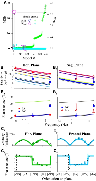
Fig. 4.
Summary of the modeling results for the VOTS neuron shown in Fig. 3. A: the normalized mean square error (MSE, left ordinate, blue-green) and Akaike information criterion weight (ωAIC; right ordinate, magenta-light blue) obtained from all successfully converged models were computed with the frequency-spatiotemporal fits. Both quantities are plotted according to the ascending order of MSE. Each model is labeled with the same marker style but different colors (e.g., the paired circles indicated by the double arrowheaded line). The simple model with the highest ωAIC (=0.65; magenta circle with arrow) also had a very low MSE (0.35, blue circle with arrow), indicating that this was the most parsimonious model of all models tested. B: comparison of actual and predicted responses from the chosen model indicated in A. Bode plots, i.e., sensitivity and phase vs. frequency, of actual (markers) and predicted (thick lines) responses, are plotted along the IA, NO, and DV axes. Estimated response dynamics in the intermediate orientations, sampled at a 15° interval, are also shown (thin lines). Note that although matching sensitivity and phase curves are graphed, only 2 stacks of phase curves are visible. C: spatial tuning curves of the same VOTS neuron in the horizontal and frontal planes. Actual (markers) response sensitivity and phase vs. translation directions are superimposed on the estimated responses from the global frequency-spatiotemporal model (solid lines). In addition, unrestricted, independent 2-dimensional fits to the horizontal and sagittal plane data are shown in dashed lines. The 2 identical peaks in the sensitivity plots correspond to peak responses in the excitatory and inhibitory directions. Error bars (SEs) in B and C are shown in one direction and may be obscured by symbols.

