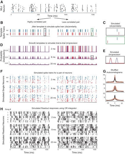
Fig. 7.

Simulating pairs of neurons with varying degrees of temporal precision and spike train similarity. A: a spike train from a real MLd neuron was used as a template from which simulated spike trains were generated. Each row shows the spiking response to one presentation of a single song; the bottom row (colored blue) was used as the template for the first simulated neuron in each pair (N1). B, D, F, and H: the left column in each panel shows a pair of neurons with highly correlated responses and the right column shows a pair of neurons with less correlated responses. B: temporal jitter was added to each “spike” in the N1 template to create a template for the second simulated neuron (N2). C: close-up of the amount of jitter introduced to the template in the left and right panels of B. D: the templates for N1 and N2 were smoothed with Hanning windows that ranged in width from 1 to 100 ms, resulting in continuous probability distributions. The blue distributions correspond to N1 and the red distributions to N2. The top, bottom, and middle panels show smoothing widths of 2, 8, and 20 ms. E: close-up of the amount of smoothing applied to the templates for N1 and N2. F: 10 spike trains were generated from each of the probability distributions. The top, middle, and bottom panels show spike trains for N1 and N2, generated from the respective distributions in D. G: the average shuffled autocorrelogram (SAC) of real MLd neurons (mean shown in black) compared with the SACs of simulated neurons (±1SD shown in red) with 2, 8, and 20 ms smoothing windows (from top to bottom). H: responses from an OR readout neurons that received simulated spike trains from N1 and N2 as inputs. From top to bottom, the readout neurons received input with progressively coarser temporal precision. Each panel shows 10 simulated responses to each of 5 songs.