Calculation of the confidence intervals for transformation parameters in the registration of medical images

Abstract

Images from different individuals typically cannot be registered precisely because anatomical features within the images differ across the people imaged and because the current methods for image registration have inherent technological limitations that interfere with perfect registration. Quantifying the inevitable error in image registration is therefore of crucial importance in assessing the effects that image misregistration may have on subsequent analyses in an imaging study. We have developed a mathematical framework for quantifying errors in registration by computing the confidence intervals of the estimated parameters (3 translations, 3 rotations, and 1 global scale) for the similarity transformation.

The presence of noise in images and the variability in anatomy across individuals ensures that estimated registration parameters are always random variables. We assume a functional relation among intensities across voxels in the images, and we use the theory of nonlinear, least-squares estimation to show that the parameters are multivariate Gaussian distributed. We then use the covariance matrix of this distribution to compute the confidence intervals of the transformation parameters. These confidence intervals provide a quantitative assessment of the registration error across the images. Because transformation parameters are nonlinearly related to the coordinates of landmark points in the brain, we subsequently show that the coordinates of those landmark points are also multivariate Gaussian distributed. Using these distributions, we then compute the confidence intervals of the coordinates for landmark points in the image. Each of these confidence intervals in turn provides a quantitative assessment of the registration error at a particular landmark point. Because our method is computationally intensive, however, its current implementation is limited to assessing the error of the parameters in the similarity transformation across images.

We assessed the performance of our method in computing the error in estimated similarity parameters by applying that method to real world dataset. Our results showed that the size of the confidence intervals computed using our method decreased – i.e. our confidence in the registration of images from different individuals increased – for increasing amounts of blur in the images. Moreover, the size of the confidence intervals increased for increasing amounts of noise, misregistration, and differing anatomy. Thus, our method precisely quantified confidence in the registration of images that contain varying amounts of misregistration and varying anatomy across individuals.

1. Introduction

Image registration is the process of spatially transforming images into a common coordinate space such that anatomical landmarks in one image match the corresponding landmarks in another image. Ideally, these landmarks match perfectly across the images. In practice, however, errors in image registration are inevitable. These errors proportionately increase the level of noise in any subsequent processing or statistical analysis of the images. For example, in functional magnetic resonance imaging (fMRI) datasets, noise in the analysis caused by error in registration of the functional images will reduce the likelihood of detecting significant task-related change in signal from the brain. Given the need to minimize error, a number of excellent methods for image registration have been proposed (Brown, 1992; Viola and Wells, 1997; Lester and Arridge, 1999; Hanjal et al., 2001; West et al., 1996). When these methods are applied in a real world setting, information specific to the imaging application determines the number of parameters of the spatial transformation, and it determines the features of the image and the cost function that will be used to estimate the optimal values of the transformation parameters. However, none of these methods can register images perfectly, for two reasons. First, variation in brain anatomy across individuals is inevitable, making perfect registration of the images impossible, even when using high-dimensional transformations of the images. Second, image registration is fraught with inherent methodological limitations and challenges, such as the need to use degrees of freedom during spatial transformation that are inadequate to provide perfect matching of image features, and difficulties in determining the global optima of the cost function for registration (Collins and Evans, 1997; Brett et al., 2001; Nieto-Castanon et al., 2003; Hellier et al., 2003; Thirion et al., 2006). Given that images cannot be registered perfectly, quantitative assessment of the accuracy of image registration is desirable to help investigators decide whether to avail themselves of any number of options that can reduce the error in registration, which includes removing images with large amounts of error from subsequent analyses.

A number of methods have been proposed to quantify error in the registration of images. These methods fall roughly into five classes: (1) This class estimates transformation parameters using images that have been transformed by known parameters and then compares the estimated parameters with the known ones. Estimated parameters will equal known parameters if the images are perfectly registered (West et al., 1997). (2) This class predicts and quantifies the error across images by computing the average of the Euclidean distances between corresponding landmarks external to a region of interest (ROI) in the registered images (West et al., 1997; Pennec and Thirion, 1997; Fitzpatrick et al., 1998). (3) This class computes the average of the Euclidean distances between corresponding landmarks within a ROI (for example, between the anterior commissure (AC) and posterior commissure (PC)) (Grachev et al., 1999). (4) This class computes the average of the Euclidean distances between corresponding edges in the registered images (Crum et al., 2004; Fox et al., 2006). In classes 2, 3, and 4, the average distance would equal zero if the images were perfectly registered. (5) Finally, this class quantifies error by computing the overlap of corresponding structures that are defined in the registered images (Rogelj et al.,2002; Jannin et al., 2006; Hellier et al., 2003). The delineated structures overlap completely if the images are registered precisely. Because the variability in anatomy across individuals cannot be quantified directly, methods in all five categories include the effects of anatomical variability on image registration when determining the accuracy of either the estimated parameters or the matching of corresponding landmarks and structures across images.

These methods for quantifying the error in image registration have two major limitations. First, they cannot precisely assess the accuracy of registration of images that have already been transformed. For example, methods that quantify error either as the average distance between corresponding landmarks or as the amount of overlap of corresponding structures across individuals, and these landmarks and overlap of a given structure may not be features of the image that are of central importance or relevance in image registration. Other structures and landmarks in the images may not match well even when the landmarks or structures specified within the registration process do match perfectly. Therefore, if the goal was to coregister entire images, precise matching of only several specific landmarks and structures, and the use of these registered structures to compute error, would underestimate the registration error across the entire image. On the other hand, the registration error may be either overestimated or underestimated if a different set of landmarks other than the set used to register the two images is used to compute the registration error. In addition, methods that use images with known amounts of misregistration obviously cannot be used to quantify error retrospectively. Furthermore, the error computed using these methods includes the error in the manual delineation of the landmarks and structures within the image. These methods alone therefore cannot precisely quantify the error in registering the images.

The second limitation in extant methods for quantifying the error in image registration is that they do not sufficiently describe the stochastic nature (Viola and Wells, 1997) of the transformation parameters, and hence they cannot precisely quantify the registration error. The estimated transformation parameters are random variables in part because voxel intensities themselves are stochastic. In addition, delineating the features used to register the images introduces error, differences in anatomy across individuals adds to error in registration, and the methods used to estimate the optimal transformation parameters are often also stochastic. We expect the estimated transformation parameters will be intercorrelated, and therefore we must estimate the multivariate distribution and compute the confidence intervals of the parameters if we are to quantify accurately and completely the error in image registration.

We have developed a mathematical framework that retrospectively quantifies the error in registration across entire images by computing the confidence intervals of the estimated parameters of a transformation. Confidence intervals specify a range of parameter values that includes the true parameters at a specified level of confidence, confidence intervals can be used to quantify the reliability of the estimated parameters (Lehmann and Casella, 1998). Our method computes confidence intervals using image intensities directly. Therefore, it does not require a user to delineate landmark points or to define the anatomical boundaries of structures within images. Using the theory of nonlinear least-squares estimation, we show that asymptotically the estimated parameters are Gaussian distributed and $\sqrt{n}$-consistent – i.e. that their standard deviation shrinks in proportion to $\frac{1}{\sqrt{n}}$ as the sample size n grows. We then use the nonlinear relationship between those parameters and the coordinates of a given landmark point within the image to compute the multivariate Gaussian distribution and the confidence intervals of the coordinates. These confidence intervals provide a quantitative measure of the registration error at the landmark point. Similar to our method, one advanced method has been proposed previously for computing the covariance matrix of the transformation parameters that have been estimated using mutual information (Bromiley et al., 2004). The covariance matrix in this approach, however, is estimated using the lower-bound estimates on the log-likelihood function, and therefore it underestimates the error in the estimated transformation parameters.

Our method, in contrast, is independent of the method used to coregister the images, and therefore images may be registered using any one of several excellent existing techniques for registration of images. Furthermore, our method estimates the covariance matrix from the data using the principles of nonlinear estimation, and therefore the estimated error is more representative of the true error in registration. We also show that estimation parameters for image registration asymptotically are Gaussian distributed. We validate our formulation using brain images from living subjects and by computing the confidence intervals for parameters of similarity transformation and for the coordinates at five landmarks points. Finally, we assess the size of the confidence intervals when noise and anatomical differences increased across the brain images acquired from 169 individuals.

2. Method

Voxel intensities within and across images of the brain are related nonlinearly to one another, and this relation can be estimated only from the joint histogram of intensities within images that are closely registered. In general, because the intensity across images from different individuals vary locally, the relation of intensities across images is not a uniquely defined function (i.e. a single intensity in one image may map to multiple intensities in another image when images are from different imaging modality). In our formulation, however, we assume a nonlinear relation between intensities across the two images, an assumption that is true for typical sets of medical images. For example, the relations between intensities across images of the brain from various MR modalities can be modeled using nonlinear functions. We should note that intensities across CT and MR images are not functionally related, however, and in this case our method may not be useful in assessing the accuracy of their estimated parameters for registration. Because various methods (Grachev et al., 1999; Hellier et al., 2003; Penney et al., 1998; Viola and Wells, 1997; West et al., 1997; Wang and Staib, 2000; Cachier et al., 2001; Johnson and Christensen, 2002) register MR images with sufficiently high accuracy, we use the joint histogram of the registered images to estimate this nonlinear function f(·) between intensities across images (Figs. 2 and 10). In general, the relation between intensities is a function, and therefore modeling the relation using a nonlinear function in our method will overestimate the variance of the transformation parameters. Given the nonlinear function f(·), and assuming a conditional Gaussian distribution of intensities because of Gaussian noise, the optimal transformation parameters minimize the sum of the square differences between the intensities in the float image and the intensity predicted by the function f(·). Therefore we use the nonlinear function f(·) and the theory of nonlinear least-squares to compute the confidence regions of the registration parameters.

Fig. 2.

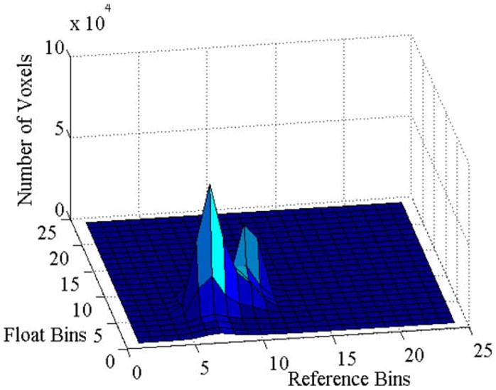
Joint histogram of intensities across the coregistered reference and float images shown in Fig. 1. Voxel intensities in each image ranged from 0 to 1000 and we formed the joint histogram with bin size 40. The X-axis and Y-axis plot the bins of intensities in the reference and the float images, respectively. The Z-axis plots the number of voxels in each bin. The joint histogram shows that the mapping between the intensities across these two registered images can be approximated by a function, and this function can be estimated from this histogram.

Fig. 10.

Effect of blurring on joint histogram of intensities. We generated float images by blurring copies of the reference image (in Fig. 1) using 3D Gaussian kernels of standard deviations 1, 2, and 4. We then formed joint histogram, with bin size 40, of intensities across the float images and the reference image. Voxel intensities in each image ranged from 0 to 1000. X-axis and Y-axis plot the bins of intensities in the reference and the float (blurred reference image) images, respectively. The Z-axis plots the number of voxels in each bin. Increasing amounts of blur increased the spread of intensities in the joint histograms. The relation between the intensities across images, however, can be approximated by a nonlinear function.

2.1. Confidence region of transformation parameters

We use the theory of nonlinear least-squares to compute the confidence intervals of the parameters of spatial transformation between images and at specific coordinates across images. Our method assumes that before computing the confidence intervals, the images have been registered using one of the excellent methods (Grachev et al., 1999; Hellier et al., 2003; Wang and Staib, 2000; Cachier et al., 2001; Johnson and Christensen, 2002; West et al., 1996) proposed in the literature. Although any one of these methods can be used to register two images, we have elected to use a method that maximizes the mutual information (Viola and Wells, 1997) across images for image registration. We then use the joint histogram of intensities to estimate the nonlinear relation f(·). We formulate the problem of quantifying the error in registration using the theory of nonlinear least-squares estimation. Second, we show that asymptotically the estimated parameters are multivariate Gaussian distributed. Third, we use the covariance matrix of the Gaussian distribution to compute Wald’s statistic, which is used to calculate the confidence region of the transformation parameters. Finally, we use a numerical method based on Parzen windows with Gaussian kernels to estimate the covariance matrix of the Gaussian distribution.

2.1.1. Least-squares formulation

Let r_i denote the intensity of the ith pixel in the reference image and s_i denote the intensity of the corresponding pixel in the float image. Let β = (T_xT_yT_zR_xR_yR_zS)′ be the column vector of the transformation parameters, and f(r_i,β) be the nonlinear function that maps intensity r_i to s_i for the specified set of parameters β. The optimal estimates β̂_N of the transformation parameters, in the nonlinear least-squares sense, are

$${\widehat{\beta }}_N={min}_{\beta }{Q}_N(\beta )={min}_{\beta }\frac{1}{N}\sum _{i=1}^N{[s_i-f(r_i,\beta )]}^2.$$

We estimate the nonlinear function f(r_i, β) as the expected value of s for a specified value r_i. The gradient of the cost function Q_N(β) is computed as

$${\nabla }_{\beta }{Q}_N(\beta )=\frac{\partial Q_N(\beta )}{\partial \beta }=\frac{2}{N}\sum _{i=1}^n[s_i-f(r_i,\beta )]\left[\frac{\partial s_i}{\partial \beta }-\frac{\partial }{\partial \beta }f(r_i,\beta )\right]$$

and the ${\nabla }_{\beta }^2{Q}_N(\beta )$ is calculated as

$${\nabla }_{\beta }^2{Q}_N(\beta )=\frac{\partial }{\partial {\beta }^{\prime }}\frac{\partial }{\partial \beta }{Q}_N(\beta )=\frac{2}{N}\sum _{i=1}^N\left\{\left[\frac{\partial s_i}{\partial \beta }-\frac{\partial }{\partial \beta }f(r_i,\beta )\right]\times {\left[\frac{\partial s_i}{\partial \beta }-\frac{\partial }{\partial \beta }f(r_i,\beta )\right]}^{\prime }+[s_i-f(r_i,\beta )]\left(\frac{\partial }{\partial {\beta }^{\prime }}\frac{\partial s_i}{\partial \beta }-\frac{\partial }{\partial {\beta }^{\prime }}\frac{\partial }{\partial \beta }f(r_i,\beta )\right)\right\}$$

The Hessian $H_N(\beta )=E[{\nabla }_{\beta }^2{Q}_N(\beta )]$ is approximated by the first-order derivatives only, i.e.

$$H_N(\beta )\approx E[{\nabla }_{\beta }^2{Q}_N(\beta )]=\frac{2}{N}\sum _{i=N}^N\left\{E\left[\left[\frac{\partial s_i}{\partial \beta }-\frac{\partial }{\partial \beta }f(r_i,\beta )\right]\times {\left[\frac{\partial s_i}{\partial \beta }-\frac{\partial }{\partial \beta }f(r_i,\beta )\right]}^{\prime }\right]+E\left[[s_i-f(r_i,\beta )]\left(\frac{\partial }{\partial {\beta }^{\prime }}\frac{\partial s_i}{\partial \beta }-\frac{\partial }{\partial {\beta }^{\prime }}\frac{\partial }{\partial \beta }f(r_i,\beta )\right)\right]\right\}=\frac{2}{N}\sum _{i=1}^{N}E\left[\left[\frac{\partial s_i}{\partial \beta }-\frac{\partial }{\partial \beta }f(r_i,\beta )\right]{\left[\frac{\partial s_i}{\partial \beta }-\frac{\partial }{\partial \beta }f(r_i,\beta )\right]}^{\prime }\right],$$

when the estimation error e_i = s_i − f(r_i, β) at a location i is uncorrelated with $\left(\frac{\partial }{\partial {\beta }^{\prime }}\frac{\partial s_i}{\partial \beta }-\frac{\partial }{\partial {\beta }^{\prime }}\frac{\partial }{\partial \beta }f(r_i,\beta )\right)$ and the second-order derivatives of the function f(·) are small. Therefore, the consistent estimator of the Hessian H_N(β) is calculated as the sample average, i.e.

$$H_N(\beta )\approx \frac{2}{N}\sum _{i=1}^2\left[\frac{\partial s_i}{\partial \beta }-\frac{\partial }{\partial \beta }f(r_i,\beta )\right]{\left[\frac{\partial s_i}{\partial \beta }-\frac{\partial }{\partial \beta }f(r_i,\beta )\right]}^{\prime }.$$

We use the consistent estimator of H_N(β) to compute the covariance matrix of the transformation parameters.

2.1.2. Transformation parameters are Gaussian distributed

Let β^* be the parameters that globally minimize the cost function E[Q_N(β)], β̂_N is the set of parameters that minimize Q_N(β), ${\beta }_N^{+}$ and are some parameters between β^* and β̂_N. Because β^* and β̂_N are expected to be close, by the mean value theorem (Rudin, 1976) the expansion of ∇_βQ_N(β̂_N) around β^* is

$${\nabla }_{\beta }{Q}_N({\widehat{\beta }}_N)={\nabla }_{\beta }{Q}_N({\beta }^{\ast })+{\nabla }_{\beta }^2{Q}_N({\beta }_N^{+})·({\widehat{\beta }}_N-{\beta }^{\ast }).$$

Furthermore, because β̂_N is the optimal estimate that minimizes Q_N(β̂_N), i.e. ∇_βQ_N(β̂_N) = 0, and because β^* and β̂_N and are close, we have

$$\begin{array}{l}\sqrt{N}({\widehat{\beta }}_N-{\beta }^{\ast })=-{[{\nabla }_{\beta }^2{Q}_N({\beta }_N^{+})]}^{-1}\sqrt{N}{\nabla }_{\beta }{Q}_N({\beta }^{\ast })\\ \approx H_N{({\beta }^{\ast })}^{-1}\sqrt{N}{\nabla }_{\beta }{Q}_N({\beta }^{\ast }).\end{array}$$ (1)

The approximation in the second equation follows from the fact that ${\beta }_N^{+}$ converges to β^* because β̂_N converges to β^* for large values of N. Therefore, $\sqrt{N}({\widehat{\beta }}_N-{\beta }^{\ast })$ is distributed according to the distribution of $H_N{({\beta }^{\ast })}^{-1}\sqrt{N}{\nabla }_{\beta }{Q}_N({\beta }^{\ast })$, which is multivariate Gaussian distributed by the Central Limit Theorem. Let $V_N^{\ast }({\beta }^{\ast })$ denote the covariance matrix of $\sqrt{N}{\nabla }_{\beta }{Q}_N({\beta }^{\ast })$, i.e.

$$\begin{array}{l}{V}_N^{\ast }({\beta }^{\ast })=\mathit{Var}\left(-\frac{2}{\sqrt{N}}\sum _{i=1}^N[{\nabla }_{\beta }{s}_i-{\nabla }_{\beta }f(r_i,{\beta }^{\ast })]·(s_i-f(r_i,{\beta }^{\ast }))\right)\\ =\frac{4}{N}\sum _{i=1}^N\mathit{Var}[({\nabla }_{\beta }{s}_i-{\nabla }_{\beta }f(r_i,{\beta }^{\ast }))·(s_i-f(r_i,{\beta }^{\ast }))]\\ =\frac{4}{N}\sum _{i=1}^{N}E[e_i^2{\nabla }_{\beta }{s}_i-{\nabla }_{\beta }f(r_i,{\beta }^{\ast }))·{({\nabla }_{\beta }{s}_i-{\nabla }_{\beta }f(r_i,{\beta }^{\ast }))}^{\prime }],\end{array}$$

where the second equation follows from the independence of the errors e_i at all voxels for the optimal parameters β^*, and

$$E(e_i^2)={\sigma }_0^2=\frac{{\sum }_i^N{e}_i^2}{N}$$

is assumed to be independent of i (homoskedasticity condition). Therefore

$$\begin{array}{l}{V}_N^{\ast }({\beta }^{\ast })=\frac{4{\sigma }_0^2}{N}\sum _{i=1}^{N}E[({\nabla }_{\beta }{s}_i-{\nabla }_{\beta }f(r_i,{\beta }^{\ast }))·{({\nabla }_{\beta }{s}_i-{\nabla }_{\beta }f(r_i,{\beta }^{\ast }))}^{\prime }]\\ =\frac{4{\sigma }_0^2}{N}\sum _{i=1}^N({\nabla }_{\beta }{s}_i-{\nabla }_{\beta }f(r_i,{\beta }^{\ast }))·{({\nabla }_{\beta }{s}_i-{\nabla }_{\beta }f(r_i,{\beta }^{\ast }))}^{\prime },\end{array}$$

which is a consistent estimator. Thus

$${(V_N^{\ast }({\beta }^{\ast }))}^{-1/2}\sqrt{N}{\nabla }_{\beta }{Q}_N({\beta }^{\ast })\to N(0,I_7).$$ (2)

Furthermore, we have

$$\begin{array}{l}{H}_N{({\beta }^{\ast })}^{-1}{V}_N({\beta }^{\ast })H_N{({\beta }^{\ast })}^{-1}={\sigma }_0^2{\left[\frac{1}{N}\sum _{i=1}^N({\nabla }_{\beta }{s}_i-{\nabla }_{\beta }f(r_i,{\beta }^{\ast })]·{({\nabla }_{\beta }{s}_i-{\nabla }_{\beta }f(r_i,{\beta }^{\ast }))}^{\prime }\right]}^{-1}\\ =D_N({\beta }^{\ast })\end{array}$$ (3)

and therefore

$${(D_N({\beta }^{\ast }))}^{-1/2}{H}_N{({\beta }^{\ast })}^{-1}\sqrt{N}{\nabla }_{\beta }{Q}_N({\beta }^{\ast })\to N(0,I_7).$$ (4)

Thus, from Eqs. (1), (3) and (4), the Gaussian distribution of the estimated transformation parameters β̂ around the optimal parameters β^* is

$${[D_N({\beta }^{\ast })]}^{-1/2}\sqrt{N}({\widehat{\beta }}_N-{\beta }^{\ast })\to N(0,I_7)$$

the covariance matrix $\widehat{\mathit{Var}}({\widehat{\beta }}_N)$ is β̂_N estimated as

$$\begin{array}{l}\widehat{\mathit{Var}}({\widehat{\beta }}_N)=\frac{1}{N}{D}_N({\beta }^{\ast })\\ ={\sigma }_0^2{\left[\sum _{i=1}^N({\nabla }_{\beta }{s}_i-{\nabla }_{\beta }f(r_i,{\beta }^{\ast }))·{({\nabla }_{\beta }{s}_i-{\nabla }_{\beta }f(r_i,{\beta }^{\ast }))}^{\prime }\right]}^{-1}.\end{array}$$ (5)

2.1.3. Calculating the confidence region of parameters for the transformation

To compute the confidence region of β^*, we first calculate the Wald’s statistic

$${({\widehat{\beta }}_N-\beta )}^{\prime }\widehat{\mathit{Var}}({\widehat{\beta }}_N)({\widehat{\beta }}_N-\beta ).$$

Because β̂_N is root-n consistent and asymptotically normal, the Wald’s statistic is asymptotically equivalent to the F-statistic, except for the factor 1/7. Therefore, if c_α denotes the 1 − α quantile of the F(7, N − 7) distribution, then the 1 − α confidence region for β^* is the set of all β for which

$${({\widehat{\beta }}_N-\beta )}^{\prime }\widehat{\mathit{Var}}({\widehat{\beta }}_N)({\widehat{\beta }}_N-\beta )\le 7c_{\alpha }.$$ (6)

We use this relation to compute the confidence region of the transformation parameters. Appendix A details our method for computing the covariance matrix $\widehat{\mathit{Var}}({\widehat{\beta }}_N)$.

2.2. Confidence region of the landmark coordinates

In images registered into a common coordinate space, the coordinates (x, y, z) of a point are transformed to new values (x_t, y_t, z_t) by the estimated parameters β̂ (Eq. (7)). Because β̂ is a random vector, the transformed coordinates (x_t, y_t, z_t) will also be a random vector. Using the relation between β̂ and (x_t, y_t, z_t), we compute the multivariate distribution that governs the random vector (x_t, y_t, z_t). We show that this distribution is multivariate Gaussian. We then use the covariance matrix of this distribution to compute the Wald statistic and the confidence region of the coordinates (x_t, y_t, z_t) in the reference image.

For coordinates in 2D images, we compute the covariance of the transformed coordinates (x_t, y_t) in two ways. First, we show that the transformed coordinates (x_t, y_t) are multivariate Gaussian distributed and analytically derive its covariance matrix. Second, we use a method based on Monte Carlo simulation to compute the covariance matrix of (x_t, y_t). Our experiments show that the covariance matrices computed by the two methods match well. Because the two covariance matrices match well, for the 3D coordinates we used the method of based on Monte Carlo simulation to compute the confidence regions of the transformed coordinates (x_t, y_t, z_t).

2.2.1. Theoretical development for coordinates in 2D images

Let (x_c, y_c) denote the coordinates of the center of a spatial transformation, and let (x_t, y_t) denote the coordinates of the location (x, y) transformed by the parameters β̂. Then the (x_t, y_t) are related to (x, y) as

$$\left(\begin{array}{l}{x}_t\hfill \\ y_t\hfill \end{array}\right)=S\left(\begin{array}{ll}cos\theta \hfill & -sin\theta \hfill \\ sin\theta \hfill & cos\theta \hfill \end{array}\right)\left(\begin{array}{l}x-x_c\hfill \\ y-y_c\hfill \end{array}\right)+\left(\begin{array}{l}{T}_x+x_c\hfill \\ T_y+y_c\hfill \end{array}\right).$$ (7)

Because in our method we use the float image that is registered and reformatted into the coordinate space of the reference image, θ ≈ 0, and therefore cos θ ≈ 1 and sin θ ≈ θ. The above relation can be rewritten as

$$\begin{array}{l}{x}_t=S(x-x_c)-S·\theta (y-y_c)+(T_x+x_c);\\ y_t=S·\theta (x-x_c)+S(y-y_c)+(T_y+y_c),\end{array}$$ (8)

where (x, y) and (x_c, y_c) are constants and the transformation parameters β = (S, θ, T_x, T_y) are multivariate Gaussian distributed. The transformed coordinates (x_t, y_t), which are linear sums of random variables, therefore will be Gaussian distributed if the product S · θ of jointly Gaussian random variables S and θ is Gaussian distributed. We show below that this in fact is true. Thus, the transformed coordinates (x_t, y_t) are also multivariate Gaussian distributed.

2.2.1.1. Normality of the product S · θ

Because the float image was reformatted into the coordinate space of the reference image using the estimated transformation parameters, the mean values μ_S and μ_θ of the transformation parameters S and θ will equal 1 and 0, respectively. Furthermore, μ_S ~ 1 and σ_S is small because most methods register images with sufficient accuracy and the ratio $\left(\frac{{\mu }_S}{{\sigma }_S}\right)$ is large; consequently, both the skew and the kurtosis excess of the product S · θ equal zero, i.e. skew(S · θ) ≈ 0 and excess(S · θ) ≈ 0 The distribution of the product S · θ therefore approaches normality if $\left(\frac{{\mu }_S}{{\sigma }_S}\right)\to \infty$ and $\left(\frac{{\mu }_{\theta }}{{\sigma }_{\theta }}\right)$ remains constant (0 in our case) (Aroian, 1947; Craig, 1936). Thus, the product term S · θ is Gaussian distributed, and the random variables (x_t, y_t) are jointly Gaussian distributed. We use the mean E[S · θ] and the Var(S · θ) of the product S · θ, computed as

$$\begin{array}{l}E[S·\theta ]={\mu }_{\theta }{\mu }_S+{\rho }_{S·\theta }{\sigma }_S{\sigma }_{\theta }={\rho }_{S·\theta }{\sigma }_S{\sigma }_{\theta },\\ \mathit{Var}(S·\theta )={\sigma }_{\theta }^2+{\sigma }_S^2{\sigma }_{\theta }^2(1+{\rho }_{S·\theta }^2)\end{array}$$

to calculate the covariance matrix Σ_xy of the transformed coordinates (x_t, y_t).

2.2.2. Computing the covariance matrix using Monte Carlo simulation

We estimate the covariance matrix of the transformed coordinates (x_t, y_t) using Monte Carlo simulation. The coordinates (x_t, y_t) are related to the transformation parameters (T_x T_y θS)′ by Eq. (7). We use the mean values and covariance matrix of the parameters (T_x T_y θS)′ to generate 100,000 simulated values from their multivariate Gaussian distribution. These simulated values of (T_x T_y θS)′ are used to generate 100,000 values for the transformation coordinates (x_t, y_t), from which we compute their sample mean ( $\overline{x_t},\overline{y_t}$) and covariance matrix Σ_sim as

$$\begin{array}{l}\overline{x_t}=\frac{1}{N}\sum _{i=1}^N{x}_t^i,\overline{y_t}=\frac{1}{N}\sum _{i=1}^N{y}_t^i,\\ \sum _{\text{sim}}=\frac{1}{N-1}\left(\begin{array}{ll}\sum {(x_t^i-\overline{x_t})}^2\hfill & \sum (x_t^i-\overline{x_t})(y_t^i-\overline{y_t})\hfill \\ \sum (x_t^i-\overline{x_t})(y_t^i-\overline{y_t})\hfill & \sum {(y_t^i-\overline{y_t})}^2\hfill \end{array}\right)\end{array}$$

2.2.3. The confidence interval of the transformed coordinates

The transformed coordinates are Gaussian distributed; therefore, the Wald’s statistic will be χ²(2) when computed using the covariance matrix Σ_xy that was computed analytically. However, when the simulated covariance matrix Σ_sim is used, the normalized Wald statistic will be distributed according to Fisher F-distribution.

2.2.3.1. Theoretical derivation

Let Σ_xy be the covariance matrix of the transformed coordinates (x_t, y_t). Then the Wald statistic

$$(x_t-x{y}_t-y)\sum _{xy}^{-1}{(x_t-x{y}_t-y)}^{\prime }$$

is χ²(2) distributed. If χ_α denotes the 1 − α quantile of the χ²(2) distribution, then the 1 − α confidence region is the set of all (xy) for which

$$(x_t-x{y}_t-y)\sum _{xy}^{-1}{(x_t-x{y}_t-y)}^{\prime }\le {\chi }_{\alpha }.$$

2.2.3.2. Monte Carlo simulation

The Wald statistic

$$(x_t-x{y}_t-y)\sum _{\text{sim}}^{-1}{(x_t-x{y}_t-y)}^{\prime },$$

computed using Σ_sim is equivalent to the F-statistic, except for the factor 1/2. Therefore, if c_α denotes the 1 − α quantile of the F(2, N − 2) distribution, then the 1 − α confidence region is the set of all (xy) for which

$$(x_t-x{y}_t-y)\sum _{\mathit{sim}}^{-1}{(x_t-x{y}_t-y)}^{\prime }\le 2c_{\alpha }.$$ (9)

2.3. Details of implementation

Calculating the confidence region of transformation parameters using our method makes extreme demands on computer time and memory. Although calculation of the covariance matrix of β̂ is not computationally intensive, to calculate the confidence region we need to find all parameters that satisfy the inequality in Eq. (6) for each significance level α. To reduce significantly the computational time and memory requirements, we computed Wald’s statistic (used to evaluate the inequality) at only 25 different values within the range of ±6 times the standard deviation of the mean value of each parameter. We selected this range of ±6 standard deviations because the multivariate distributions have more probability mass in their tail than does a univariate distribution. Therefore, sampling the parameters in the range of ±6 times the standard deviation ensured that we nearly sampled the entire confidence region of the parameters. This sampling required us to compute the Wald statistic for 25⁷ = 6 × 10⁹ different combinations of the parameter values, requiring 9 h of compute time on a 3.4 GHz PC. Although this is a coarse sampling of the parameter space, the estimated confidence regions were sufficiently accurate.

The confidence interval of a parameter is obtained by projecting the confidence region R onto the coordinate axis of that parameter. Our confidence region R in the seven-parameter space assigns a value of (1 − P) to each point sampled in the seven-parameter space, where P is the probability value computed using Wald statistic at that point. The null hypothesis used to determine the P-value for a set of transformation parameters is that β^* = β̂. For example, to obtain the confidence interval of the parameter T_x, we project R onto the axis of T_x in the parameter space: at a specific value of T_x, the projection operator π(R, T_x) assigns the smallest value in R for any combination of the other parameters with T_x set equal to the specified value. That is

$$\pi (R,T_x)=arg{min}_{\beta \mid T_x}R,$$

where β|T_x denotes that the minimum is computed for all parameters in β except for T_x, which is set equal to the specified value.

The accuracy of the estimated confidence region depends on the bin size of the joint histogram of intensities. We use the joint histogram to compute the nonlinear function f(·) and its derivatives. In the joint histogram, we set the bin size equal to 7, which we have found empirically generates the best estimates of the function f(·) and its derivatives. To ensure that this bin size works well for any set of images, we scaled the voxel intensities independently in each image within the range from 0 to 1000. We therefore could apply our methods to all images without any adjustment of the bin size. Furthermore, to ensure that estimates of the function f(·) and its derivatives are stable, we used only those bins that had greater than 200 samples of intensities from the float image. Thus, the effect of bin size was minimal on the estimated confidence regions.

3. Testing our algorithm

We tested the efficacy of our mathematical framework in computing confidence intervals whose size varied predictably for varying amounts of noise, blur, and registration errors, and for differing anatomy across individuals. These tests included three sets of experiments using 2D and 3D brain images from healthy individuals. The images were of good quality, having high signal-to-noise and contrast-to-noise ratios. To prepare images for our experiments, we preprocessed each image independently to (1) remove inhomogeneities in voxel intensities (Sled et al., 1998), (2) isolate brain from nonbrain tissue, and (3) rotate and reslice the brain into a standard orientation, such that the AC and PC landmark points were within the same axial slice. The brains were reformatted into the standard orientation using trilinear interpolation. Finally, we scaled the voxel intensities in each image to fall within the range of 0 to 1000. We selected at random one image as the reference and estimated the parameters for the similarity transformation that best registered other images to the reference by maximizing mutual information (Viola and Wells, 1997) across the registered images. The centers of the image volumes were set as the origin of the transformation between the two images. The registered images were then resliced into the coordinate space of the reference using the estimated parameters. The resliced, registered image (the float) and the reference image were used in our experiments as described below.

The sizes of the confidence intervals computed using our method depended upon many factors. For increasing amounts of noise, misregistration, and differing anatomy across images, we expected the size of the confidence intervals to increase, thereby accurately quantifying our decreasing confidence in the registration of the images. However, for increasing amounts of blur, the definition of anatomy will become less precise. As a consequence, anatomical differences will increase across images from a single individual, but they will decrease across images from differing individuals. Therefore, for increasing amounts of blur, we expected our method to compute confidence intervals that increased in size for images from a single individual but decreased for images from different individuals, thereby accurately quantifying our confidence in the registration of the images in the presence of blur.

We first computed confidence intervals using images from a single individual. In these experiments, we generated synthetic float images by introducing increasing amounts of translation, rotation, scaling, and blurring into copies of the reference image. The images were blurred using isotropic Gaussian kernels of varying standard deviation. Because the simulated float images that were not blurred contained anatomical information identical to that of the reference image, changes in the confidence intervals would reflect the effects of misregistration alone on the computed confidence intervals.

In the second set of experiments, we used images from two different individuals to demonstrate that our method computed confidence intervals as we expected for increased level of complexity in real world. In these experiments, we generated simulated float images by introducing increasing amounts of translation, rotation, scaling, and blurring into copies of the float image. Because anatomy differed across the reference and float images, we expected the confidence intervals to be larger in these experiments than those generated using copies of images from a single individual. We also expected our method to compute larger confidence intervals for larger amounts of misregistration across images. Increasing amounts of blur reduces variability in anatomical definitions across images, however, and therefore we expected the confidence intervals to decrease for increasing amounts of blur across images from different individuals.

Finally, in a third set of experiments we demonstrated that the confidence intervals computed using our method increase for increasing amounts of noise and differing anatomy. We computed confidence intervals for the coordinates of the anterior commissure in a set of 169 brain images. Each image in this set was registered assuming similarity transformation to the reference image using a similarity transformation such that mutual information was maximized across images. We expected larger confidence intervals in images with larger amounts of noise, motion artifact, and variability in anatomy.

3.1. Image acquisition protocol

The high-resolution T1-weighted MR images were acquired with a single 1.5-T scanner (GE Signa; General Electric, Milwaukee, WI) using a sagittal 3D volume spoiled gradient echo sequence with repetition time = 24 ms, echo time = 5 ms, 45° flip angle, frequency encoding superior/inferior, no wrap option, 256 × 192 matrix, field of view = 30 cm, two excitations, slice thickness = 1.2 mm, and 124 contiguous slices encoded for sagittal slice reconstruction, with voxel dimensions 1.17 × 1.17 × 1.2 mm.

3.2. 2D Analysis

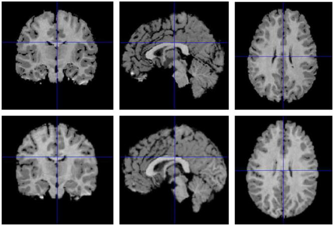
In these analysis, we selected as the 2D reference image a single axial slice (slice number 50, Fig. 1) from the 3D volume of the reference image. The corresponding slice from the 3D float volume was used as the 2D float image. We used these images to compute the confidence intervals of the affine parameters and of the coordinates of the top left-most point in the reference image. The confidence interval of the coordinates was computed in two ways: theoretically, and using Monte Carlo simulation. We compared the two confidence intervals that were computed in these two ways to assess the accuracy of our Monte Carlo simulations in calculating the confidence intervals.

Fig. 1.

Three orthogonal views through the brain images of two individuals used in our 3D analysis. The brain image of one individual was selected as the reference image (top row). The brain image of the other individual was registered and resliced into the coordinate space of the reference by maximizing mutual information (Viola and Wells, 1997) across images. The resliced image is called the float image (bottom row). The right column shows the two axial slices (slice number 50) used in our 2D analysis. The X-axis is left to right, the Y-axis is posterior to anterior, and the Z-axis is inferior to superior of the brain.

3.3. 3D Analysis

Confidence intervals are stochastic because they are computed from the covariance matrix of the multivariate Gaussian distribution estimated from a finite sample of voxel intensities. However, because the estimated covariance matrix is consistent, we expected that our method would compute confidence intervals of affine parameters that converge for a larger number of samples from 3D images and that therefore yield a more valid analysis of the effects of misregistration and differing anatomy on confidence intervals.

3.4. Confidence region of landmarks in MR images from two individuals

Our method computes confidence intervals while accounting for differing anatomy and misregistration across images; we therefore expected landmarks in the float image to be within the confidence interval of the corresponding landmarks identified in the reference image. To assess the accuracy of the confidence intervals computed using our method, an expert delineated five landmarks in the reference image and the corresponding landmarks in the float image. These five landmarks were: the AC and PC points, the most anterior point of the genu of the corpus callosum, a point on the dorso-lateral aspect of the prefrontal cortex (DLPFC), and a point in the occipital cortex (OC). We selected these landmarks because they can be identified reliably across images from individuals with differing anatomy. We expected that the size of the confidence intervals computed using our method would be small for the AC, PC, and genu because they were close to the origin of transformation. However, because the DLPFC and OC points were located on the surface of the cortex, and therefore were comparatively farther from the origin of transformation, we expected the size of the confidence intervals at these points would be larger than those at the AC and PC points.

3.4.1. The AC and PC points

The AC and PC are bundles of white matter fibers that connect the two hemispheres of the brain across the midline. These are key landmarks because they can be defined unambiguously in anatomical MR images. In the midline slice, the PC point was identified as the centermost point of the PC, and the AC point was identified as the most superior point on the AC. The coordinates of the AC point were 73, 59, 72 in the reference and 73, 61, 72 in the float image. For the PC point, the coordinates were 72, 82, 70 in the reference and 72, 81, 72 in the float image. The coordinates of various points are specified in the coordinate space of our images reformatted in the standard orientation.

3.4.2. The genu of the corpus callosum

The genu is the anterior portion of the corpus callosum. We identified its anterior-most extremity unambiguously at the midline of coronal images. The coordinates of this point were 74, 36, 64 in the reference and 74, 35, 67 in the float image.

3.4.3. The DLPFC and OC points

These were identified manually on the surface of the cortex by two experts in neuroanatomy. The DLPFC point was centered over the inferior frontal gyrus, in the mid-portion of the pars triangularis. The OC point was centered on the lowermost portion of the occipital lobe immediately to the left of the interhemispheric fissure, such that the medial edge of the spherical deformation was tangential both to the interhemispheric fissure and the cistern immediately superior to the cerebellum. We have shown elsewhere that these points can be identified with high inter-rater reliability across images from different individuals (Bansal et al., 2005). The coordinates of the DLPFC point were 118, 34, 69 in the reference and 119, 40, 66 in the float image. For the OC point, the coordinates were 86, 143, 76 in the reference and 81, 143, 77 in the float.

3.5. Effect of differing anatomy on confidence intervals

We showed that the size of the confidence intervals increased for increasing amounts of noise and differing anatomy. We computed confidence intervals using our high-resolution, T1-weighted MR images from 169 different individuals. This group of 169 individuals included 76 males and 93 females, with ages ranging from 6 to 72 years. We selected one image (Fig. 16a) as the reference based on its high quality and because the individual’s demographics were representative of the demographics of the group as a whole. We registered the other 168 brains to this reference brain using a method that mutual information (Viola and Wells, 1997) assuming a similarity transformation across images. To test the accuracy of image registration, we identified and compared coordinates of the AC point in each of these 169 registered brains. Because the AC was identified in the individual brains registered to the reference, we expected that the absolute values of the difference between the coordinates to equal zero in the reference and registered brains. We then used our method to compute the confidence interval of each coordinate of the AC for every brain. Because the brains were well registered, we expected that the confidence intervals would be small and would not correlate with the differences in the coordinates of the AC point. Differences in the confidence intervals therefore would be caused by differing anatomy across individuals in the group. We expected our method to compute larger confidence intervals for images with larger amounts of noise and differing anatomy.

Fig. 16.

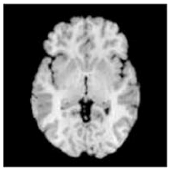
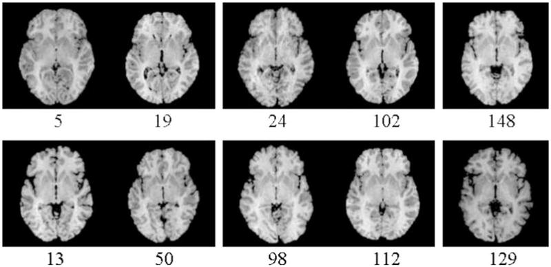
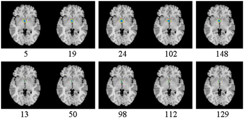
Fig. 16a. The reference brain used to study of the effect varying anatomy on the estimated confidence region for the coordinates of the AC and PC. The reference brain was rotated into the Talairach space and the axial slice containing the AC and PC is shown.

Fig. 16b. Differences versus 68.5% confidence intervals of the X-, Y-, and Z-coordinates of the AC point delineated in the reference and 168 brains registered to the reference. Differences in the coordinates of the AC identified in the reference brain and the other 168 brains are plotted against their confidence intervals. Differences in the X and Z-coordinates are small, indicating that the images are well registered along the left to right and inferior to superior directions. Larger differences in the Y-coordinate are indicative of the anatomical variability along the anterior–posterior direction across individuals. Because the brains were well registered to the references, differing confidence intervals are caused by differing anatomy and differing amounts of noise across individuals. On the other hand, the confidence intervals did not correlate with the differences in coordinates because of the inaccuracies in identifying manually the AC across individuals.

Fig. 16c. Axial images through the AC–PC plane in a representative set of 10 individuals before they were registered to the reference brain (Fig. 16a). In the images registered to the reference image, we computed the differences in X-, Y-, and Z-coordinates of the AC point in the individual and the reference images. The difference was ±1 voxels for the X- and Z-coordinates, and ±2 voxels for the Y-coordinate. The images in the top row have larger amounts of both motion artifacts and noise than the images in the bottom row.

Fig. 16d. Confidence region of the coordinates of the AC for 10 example individuals (Fig. 16c). The confidence regions are superimposed on the slice 73 (slice containing the AC and PC) from the reference image (Fig. 16a). Blue: region of 68.5% confidence; green: region of 95% confidence; orange: region of 99% confidence. In the images numbered 5, 19, 24, 102, and 148 (top row), the average 68.5% confidence intervals of the X-, Y-, and Z-coordinate were ±3.93, ±3.21, and ±1.91 voxels, respectively. In images numbered 13, 50, 98, 112, and 129 (bottom row), the average 68.5% confidence intervals were ±1.8, ±2.0, and ±1.55 voxels for the X-, Y-, and Z-coordinates. The images in the top row have larger amounts of both motion artifacts and noise than the images in the bottom row. Confidence regions are larger for images with larger amounts of noise and differing anatomy than the reference image. (For interpretation of the references to colour in this figure legend, the reader is referred to the web version of this article.)

4. Results

4.1. Distribution of Wald’s statistics

The product random variable S × θ is Gaussian distributed (Fig. 3). Therefore, the transformed coordinates of a point are multivariate Gaussian distributed, and the normalized Wald’s statistic is distributed according to Fisher F-distribution. Thus we used the normalized Wald statistics to compute the confidence intervals of the coordinates.

Fig. 3.

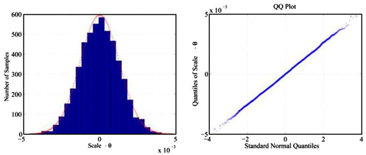
Scale · θ is Gaussian distributed. We sampled values of S and θ from their joint multivariate Gaussian distribution and computed product of the values. From a sample of the product values and a sample of values from the standard Gaussian distribution, we generated the histogram (left) and the quantile–quantile (QQ) plot (right). The red line in the histogram displays the Gaussian distribution whose variance equals the variance of the sample of product values. Both the histogram and the QQ plot show that the distribution of the product values S · θ closely follows a Gaussian distribution. (For interpretation of the references to colour in this figure legend, the reader is referred to the web version of this article.)

4.2. Monte Carlo simulation

In these experiments, we used Monte Carlo simulation to compute the confidence intervals of the coordinates of the top left-most point in the reference image. These confidence intervals were computed using the reference image and simulated float images with varying amounts of blur and misregistration. Confidence intervals computed using this method (Fig. 7) matched well those calculated using our theoretical formulation (Figs. 6a and 6b), thus demonstrating that Monte Carlo simulation is sufficiently accurate to compute precisely the confidence intervals of coordinates of points in 3D images.

Fig. 7.

Using Monte Carlo simulation to estimate the confidence intervals of the coordinates (0, 0) for increasing amounts of (i) translation along the X-axis, (ii) rotation about the Z-axis, (iii) scale, and (iv) blur in copies of the float image. The confidence intervals for X- and Y-coordinate, X- and Y-translation, and X-shift are in voxels. These intervals match well with those estimated using our theoretical formulation (Fig. 6a and 6b). We therefore use Monte Carlo simulation to estimate the confidence intervals for the coordinates (0, 0, 0) in our 3D analysis.

Fig. 6.

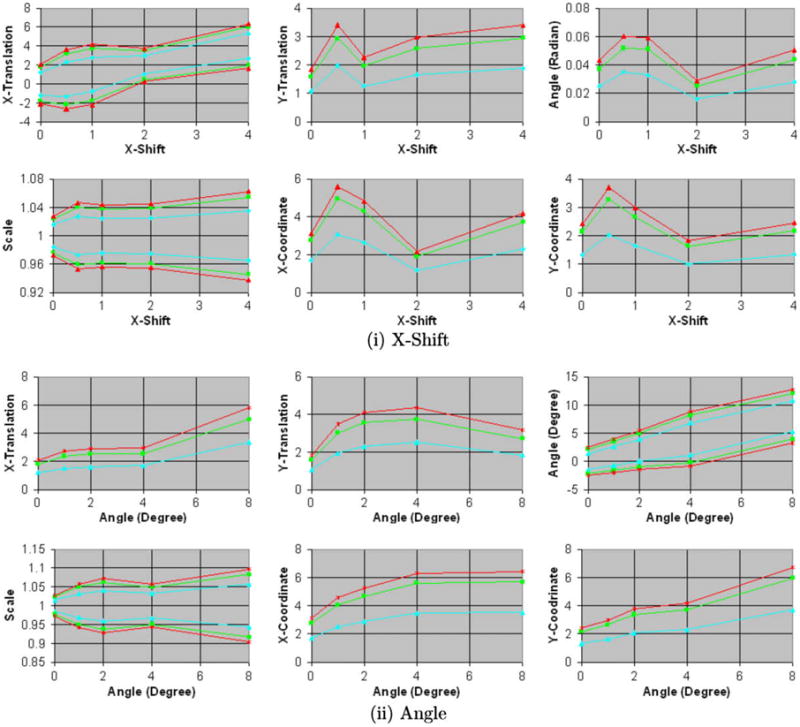
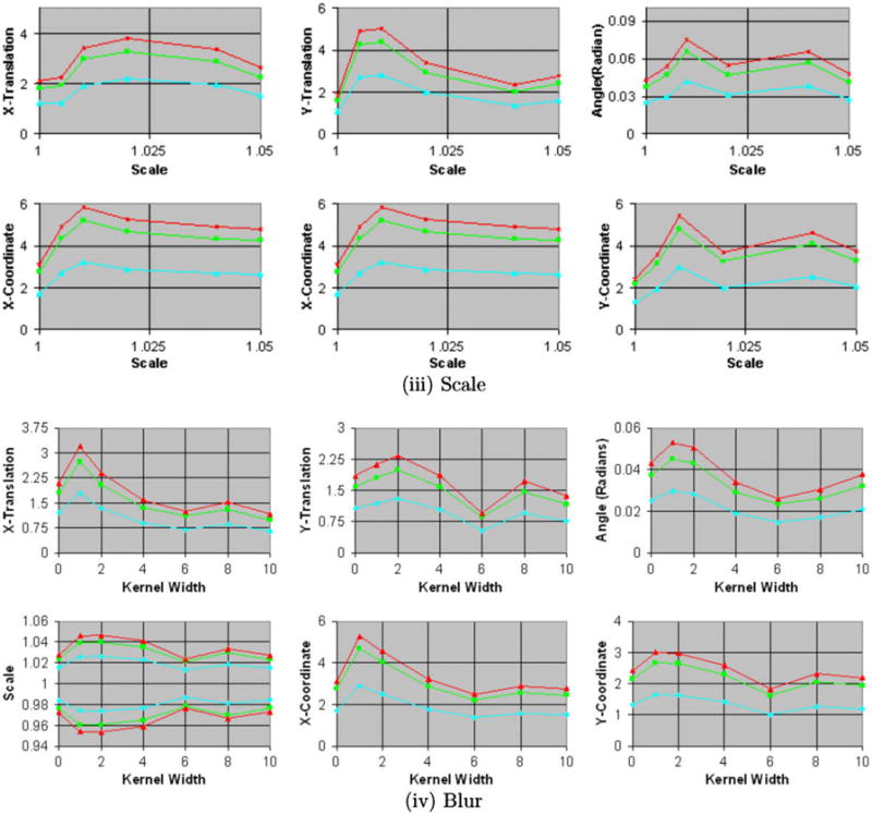
Fig. 6a. Confidence intervals of the coordinates (0, 0) and parameters for similarity transformation using image from two individuals. The confidence intervals for X- and Y-coordinate, X- and Y-translation, and X-shift are in voxels. Simulated float images were generated by (i) translating and (ii) rotating by increasing amounts the copies of the float image. The size of the confidence regions increases for increasing amounts of misregistrations and is larger than those estimated using images from single individual (Fig. 5a). Blue: region of 68.5% confidence; green: region of 95% confidence; and orange: region of 99% confidence. For the confidence intervals that are symmetric around 0.0, only the upper limits are shown. (For interpretation of the references to colour in this figure legend, the reader is referred to the web version of this article.)

Fig. 6b. Confidence intervals generated using simulated float images for increasing amounts of (iii) scale and (iv) blur in copies of 2D float images. The confidence intervals for X- and Y-coordinate, X- and Y-translation, and X-shift are in voxels. The size of confidence intervals tends to decrease for increasing amounts of blur in the simulated float images.

4.3. Images from a single individual

The confidence intervals of the parameters of similarity transformation, as well as the (0, 0) coordinates in 2D and 3D analyses, were smaller than a single voxel when the confidence intervals were computed using identical copies of the reference brain (Figs. 4 and 8). Thus, based on confidence intervals computed using our method, we could correctly conclude that the images were registered with high precision.

Fig. 4.

Ellipsoids of the confidence regions for the parameters of 2D similarity transformation (left and middle) and the coordinates (0,0) (right). The confidence regions were estimated using identical copies 2D reference image (top-right image in Fig. 1). For transformation parameters, we first computed confidence region in the four-dimensional space of the parameters, and then projected the region on the 2D parameter spaces of the X-translation and Y-translation (left), and the scale and theta (middle). Blue: region of 68.5% confidence; green: region of 95% confidence; and orange: region of 99% confidence. Because we used identical copies of the reference image, the confidence regions are less than a pixel wide. (For interpretation of the references to colour in this figure legend, the reader is referred to the web version of this article.)

Fig. 8.

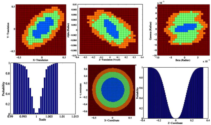
Confidence regions of the parameters of the 3D similarity transformation and X-, Y-, and Z-coordinates (0, 0, 0) estimated using identical copies of the 3D reference image. The confidence intervals for X-, Y- and Z-coordinate, X-, Y- and Z-translation, and X-shift are in voxels. The confidence intervals for the transformation parameters and the coordinates are within one voxel. Because we subsampled the space of transformation parameters, the confidence regions of the transformation parameters are of lower resolution than those for the X-, Y-, and Z-coordinates. Blue: region of 68.5% confidence; green: region of 95.0% confidence; orange: region of 99.0% confidence. Small confidence regions accurately quantify our confidence that the images are precisely registered. (For interpretation of the references to colour in this figure legend, the reader is referred to the web version of this article.)

For increasing amounts of blur, X-shift, and rotation in the simulated float images, the size of the confidence intervals increased, as expected (Figs. 5a, 5b, and 9). The true transformation parameters fell within the 68.5% confidence intervals. Increasing the amounts of blur in the images increased the anatomical differences across simulated float images and the reference image, thereby decreasing our confidence in the precision of image registration. This decline in confidence was reflected by an increase in the size of the confidence intervals for the transformation parameters (Fig. 5b), which is reflective of increasing amount of spread of intensities in the joint histogram of the images (Fig. 10). These results demonstrated that our method computed confidence intervals whose size varied as expected for varying amounts of misregistration and blur in images from single individual, thus validating our method for computing the confidence intervals of the transformation parameters.

Fig. 5.

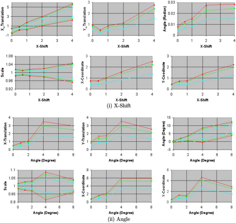
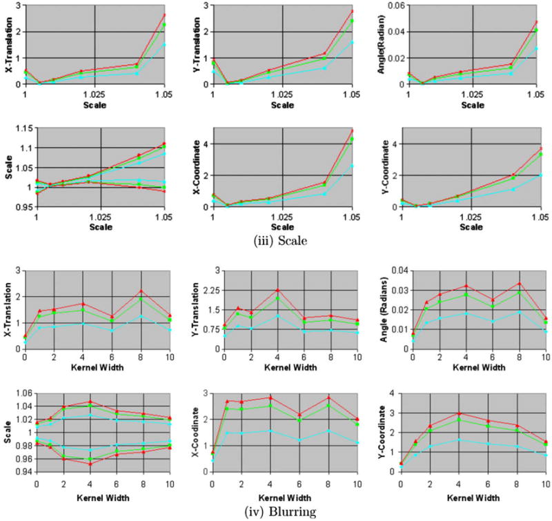
Fig. 5a. Confidence intervals of similarity parameters and X-, Y-coordinates (0, 0) for increasing amounts of X-shift and rotation of copies of the 2D reference image. The confidence intervals for X- and Y-coordinate, X- and Y-translation, and X-shift are in voxels. Copies of the 2D reference image were (i) shifted along the X-axis and (ii) rotated about the Z-axis by increasing amounts. The confidence intervals increased for increasing amounts of misregistration. Blue: region of 68.5% confidence; green: region of 95% confidence; and orange: region of 99% confidence. Only the upper limits are shown for the confidence intervals that are symmetric around 0.0. (For interpretation of the references to colour in this figure legend, the reader is referred to the web version of this article.)

Fig. 5b. Confidence intervals for increasing amounts of scale and blur. The confidence intervals for X- and Y-coordinate, X- and Y-translation, and X-shift are in voxels. In these experiments, we generated the simulated float images from copies of the 2D reference image for increasing amounts of (iii) scale and (iv) blur. The images were blurred using Gaussian kernels of increasing width specified as the standard deviation of the kernel. The size of the confidence intervals increases for increasing amounts of scale. For varying amounts of blur, the size increases for small amounts of blur and then decreases for larger amounts of blur.

Fig. 9.

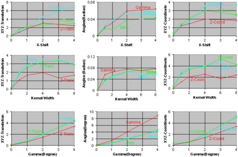
68.5% Confidence intervals for increasing amounts of misregistration in 3D images from single individual. Simulated float images were generated from copies of the reference image by adding increasing amounts of (i) translation along the X-axis, (ii) blur, and (iii) rotation about the Z-axis. The confidence intervals for the parameters of the similarity transformation and coordinates (0, 0, 0) are plotted. The images were blurred using 3D Gaussian kernel with increasing width, which was defined as the standard deviation of the Gaussian kernel. For increasing amounts of blur (second row of images), the size of confidence intervals initially increased and then remained constant for large amounts of blur. The small confidence regions accurately quantify our confidence that the images are precisely registered.

4.4. Images from two individuals

As expected, the size of the confidence intervals increased with increasing amounts of misregistration (i.e. with increasing translation, rotation, and scaling) in the simulated float images from different individuals (Figs. 6a and 11). Increasing amounts of blur, however, initially had the opposite effect of reducing the size of the confidence intervals (Figs. 6b and 11) because it reduced the anatomical differences across the reference and the simulated float image. The confidence intervals did not increase linearly with increasing scale and instead seemed to converge to a certain size for large scale. For increasing amounts of blur, the confidence intervals initially decreased for kernel widths up to 6–7 voxels (7.2–8.4 mm) and then increased for wider kernels. Therefore, initially blurring images reduced the anatomical differences between the two individuals increasing our confidence in the image registration, which was reflected by smaller confidence intervals. Larger amounts of blur, however, substantially degraded the anatomical definitions thereby decreasing our confidence in the image registration, which was quantitatively reflected by larger confidence intervals. Furthermore, these results suggest that a smoothing of about 8 mm may be optimal to register images from different individuals, a finding that is consistent with those in studies that found a smoothing kernel of width = 8 mm to be optimal for smoothing functional MRI datasets (Kiebel et al., 1999; Fransson et al., 2002). Thus, our method computed confidence intervals that varied as expected for increasing amounts of blur and varying scale, while also reflecting unexpected, nonlinear variation with differing levels of blur.

Fig. 11.

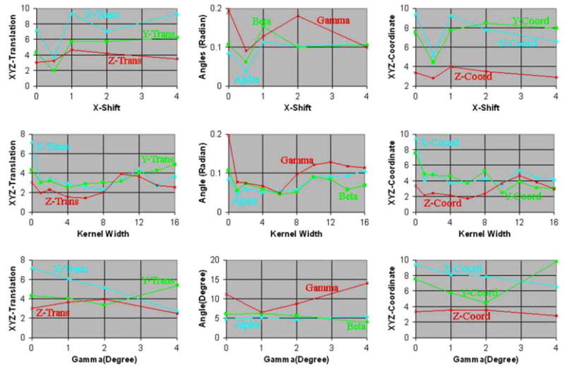
68.5% Confidence intervals for increasing amounts of misregistration using images from two individuals. Simulated float images were generated for increasing amounts of (i) translation along the X-axis, (ii) blur, and (iii) rotation about the Z-axis in the copies of the float image. We estimated the confidence intervals for the parameters of the similarity transformation and the coordinates (0, 0, 0) in the reference image. For increasing amounts of blur, the confidence intervals initially decreased for kernel widths up to 6–7 voxels (7.2–8.4 mm) and then increased for wider kernels.

4.5. Confidence intervals of landmark points

We found that the differences in the X-, Y-, and Z-coordinates of the AC and PC points across these two individuals were less than two voxels (Table 1). This result indicated that the float image was well registered to the reference image and it suggests that the increase in confidence intervals of these landmark points compared with those for copies of an image from a single individual (Fig. 12) reflects differences in anatomy across these individual images. The large difference in the coordinates for the DLPFC and OC points likely reflected a combination of operator error in locating the corresponding point on brain images (more difficult with these points than with the AC, PC, and genu), differences in anatomy across images, and errors in registration. Because the origin of transformation was located at the center of the imaging volume and because the DLPFC and OC points were on the surface of the brain (Fig. 14), far from the origin, even small amounts of misregistration would have caused disproportionately large differences in the coordinates of the corresponding points. As expected, confidence intervals for the coordinates of the genu, which was closer to the origin of transformation, was smaller than the confidence intervals for the DLPFC and OC points but larger than those for the AC and PC (Fig. 13). Therefore, the confidence intervals computed using our algorithm was larger for points further away than points closer to the origin of transformation because of imprecision in the registration of images, irrespective of differences in anatomy across images. Furthermore, corresponding points in the float image were within the 68.5 interval. In contrast, for identical copies of the reference image, our method computed confidence intervals that were less than a voxel in size at the DLPFC and OC points (Fig. 15), thereby accurately quantifying our high confidence that the images are precisely registered.

Table 1.

Coordinates and their confidence intervals of the AC, PC, genu, DLPFC, and OC points across images from two individuals.

	Differences in coordinates			68.5% Confidence intervals (voxel)			95% Confidence intervals (voxel)
	X	Y	Z	X	Y	Z	X	Y	Z
AC	0	2	0	4.74	2.67	1.98	6.87	3.87	2.87
PC	0	1	2	4.4	2.6	1.94	6.3	3.77	2.81
Genu	0	1	3	4.6	2.6	2.6	6.7	3.7	3.8
DLPFC	1	6	3	5.3	3.08	2.8	7.7	4.4	4.09
OC	5	0	f	5.23	2.6	2.15	7.5	3.8	3.12

Fig. 12.

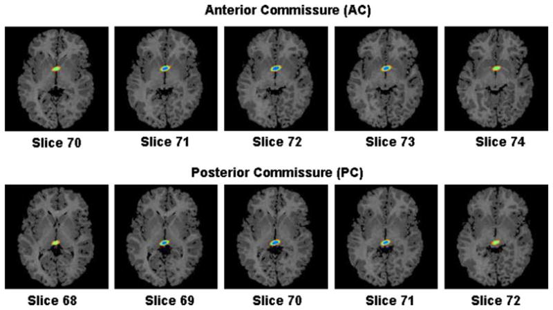
Confidence region of the coordinates of the anterior- and posterior-commissure. Coordinates of the AC and PC were (73, 59,72) and (72, 82,70) in the reference image, and (73, 61,72) and (72,81,72) in the float image. The confidence regions are displayed on axial slices from the reference image. Blue: 68.5% confidence region; green: 95.0% confidence region; orange: 99.0% confidence region of finding the AC and PC in the float image. The AC and PC in the float image are within their respective 95% confidence intervals. (For interpretation of the references to colour in this figure legend, the reader is referred to the web version of this article.)

Fig. 14.

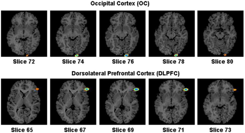
Confidence region of the coordinates of the DLPFC and OC points computed using the float image registered to the reference image. In the reference image, the coordinates of the DLPFC and OC points were (118,34,69) and (86,143,76), and in the float image the coordinates were (119,40,66) and (81,143,77), respectively. The 99% confidence regions for the two points spanned nine slices within the reference image.

Fig. 13.

Confidence region of the coordinates of the genu. The coordinates of the genu in the reference and the float images were (74, 36,64) and (74, 35,67), respectively. The confidence regions are superimposed on axial slices at the genu point in the reference image. The genu in the float image is within the 99% confidence region around the genu in the reference image.

Fig. 15.

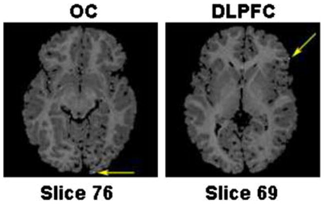
Confidence regions of the coordinates of the DLPFC and OC points computed using identical copies of the reference image. The 99% confidence regions for both points are smaller than a voxel, the white voxels pointed at by the yellow arrows. These confidence regions correctly quantify our confidence that the images are precisely registered. (For interpretation of the references to colour in this figure legend, the reader is referred to the web version of this article.)

Our method computed confidence intervals that are conservative. Although the 99% confidence intervals of the coordinates were much larger than their displacements (Figs. 12–14), the 68.5% confidence intervals more accurately reflected the magnitude of this displacement. The 68.5% confidence regions of the landmark points were as large as the width of the sulci or gyri in the image. This was expected because corresponding landmarks could be displaced by this amount in brain images from different people. Thus, although our confidence intervals were conservative, they nevertheless accounted for differing anatomy, amounts of noise and blur, and misregistration across images.

4.6. Effects of varying anatomy across individuals

The absolute values of the differences in the X- and Z-coordinates of the AC were less than 3 for most images (Fig. 16b). Because the AC was identified in the slice through the midline, the small difference in the X-coordinate shows that the midline matched well at the AC and PC across brains. Furthermore, the small difference in the Z-coordinate shows that the axial plane that intersects the AC and PC points also matched well across brains. The large differences in the Y-coordinates are attributable to anatomical differences across brains: (1) the reference brain was more spherical in shape than the other brains and (2) the varying size of the ventricles in turn varied the position of the AC along the anterior–posterior axis. The images therefore were well registered to the reference brain, with the variability in confidence intervals reflecting variability in brain anatomy across individuals. The size of the confidence intervals, however, did not correlate with the difference in the coordinates because of the variability in the manual identification of the AC across images (Fig. 16b). The confidence intervals were larger for images that had some motion artifact and noise, as well as for images with differing anatomy (top row of images, Fig. 16c) than confidence intervals for images that had less noise and motion artifact (bottom row of images, Fig. 16c). For the top row of images in Fig. 16c, the average 68.5% confidence intervals for the X-, Y-, and Z-coordinates were ±3.93, ±3.2, and ±2.3 voxels, respectively. For the other images (bottom row of Fig. 16c), the average 68.5% confidence intervals for the X-, Y-, and Z-coordinates of the AC were ±1.88, ±2.26, and ±1.89 voxels, respectively (Fig. 16d). Thus, as expected, the confidence intervals computed using our algorithm increased for increasing levels of noise and increasing anatomical differences, thereby helping to validate our method for computing the confidence intervals of transformation parameters and coordinates of landmark points.

5. Discussion

We have developed a mathematical framework for quantifying the errors in image registration. Our method uses the theory of nonlinear least-squares estimation to show that the transformation parameters are multivariate Gaussian distributed. We used the covariance matrix of the Gaussian distribution to compute the confidence intervals of the transformation parameters. We then used the nonlinear relationship between the transformation parameters and the coordinates of a landmark point to compute the multivariate Gaussian distribution and the confidence intervals of the coordinates. As expected, our method generated confidence intervals whose magnitude declined with increasing blur in images from different individuals, although the decline was nonlinear. Moreover, confidence intervals increased with increasing noise, misregistration, and anatomical differences across images. In addition, our method for quantifying error is independent of the method used for coregistering images, i.e. the images could have been coregistered using any one of the excellent methods from the field of medical image processing and our method could still be used to quantify the error in registration. Thus, our method correctly accounted for differing anatomy across individuals as well as for blur, noise, and misregistration in the images, reflecting and quantifying reasonably our degree of confidence in image registration.

The size of the confidence intervals computed using our algorithm depended upon an interplay of four sometimes competing factors: (1) anatomical differences, (2) the amount of blur present, (3) the degree of misregistration, and (4) noise level. Increasing rotation, for example, caused more voxel intensities to be interpolated, thereby increasing the amount of blur in the simulated float images. Therefore, although the confidence intervals would tend to increase with increasing rotation, the increasing blur that accompanies registration across greater rotational angles would tend to reduce the confidence intervals. Thus, the combined effect of rotation and blur could attenuate the increase associated with rotation, or even decrease the size of the confidence intervals with a sufficient level of blur. In addition, because the parameters for perfect registration are generally unknown in practice, the increasing misregistration could actually improve the registration images across individuals, thereby reducing the confidence intervals for increasing misregistrations. Thus, the interaction between differing anatomy across subjects, blur and noise in the images, and misregistration determines the size of the confidence intervals of the transformation parameters.

Increasing blur in an image causes a progressively poorer definition of anatomy. When the images to be registered were copies of the image of a single individual, increasing blur reduced the anatomical similarities and therefore the accuracy of registration that was based on the similarity of anatomy across images. Our algorithm correctly reflected this altered anatomical similarity by computing larger confidence intervals for the estimated registration parameters. When the images to be registered were from two different individuals, however, increasing blur using smoothing kernels of width up to 8 mm increased anatomical similarities (or, equivalently, it reduced anatomical differences) across images. Reducing anatomical differences in turn increased our confidence in the accuracy of image registration, which our method accurately quantified as smaller confidence intervals. Further increases in the amount of blurring, however, severely altered the anatomy in each image and across images, thereby decreasing our confidence in the accuracy of image registration. Thus, our method distinguished and correctly described the differing effects of blurgin on the registration of images that derived from one or two individuals.

Our finding that confidence in the estimated registration parameters increased for increasing amounts of blur across images from different individuals suggests that varying amounts of blur can be used to register more precisely images from different individuals. Indeed, scale-space methods register images iteratively with varying amounts of blur (ter Haar Romeny and Florack, 1993; Florack et al., 1992; Fritsch, 1993; Pizer et al., 1994; Romeny et al., 2001; Eldad et al., 2005). In the initial iterations, images with large amounts of blur are used to estimate transformation parameters. The parameters estimated in that iteration then are used as the initial estimates for the next iteration for images with lesser amounts of blur. The intuition behind these methods is that blurring of images reduces local minima in the cost function and therefore helps the method to converge to a globally optimal set of parameters. Our method provides quantitative support for the value of these scale-space methods. For larger amounts of blur, not only are fewer local minima present in the cost function, but also the registration parameters are estimated with greater accuracy. A greater accuracy of registration parameters in the initial iterations with large amounts of blur can help to guide the scale-space methods to converge on a more globally optimal set of registration parameters more accurately and more efficiently.

Our method can be used to control the quality at the many levels of automatic, post-acquisition processing of images. Images are generally registered initially and in several levels of postprocessing. Errors in registration can seriously affect the accuracy of subsequent image processing and statistical analyses. Our method provides a quantitative assessment of error in image registration by providing confidence intervals for the parameters of transformation. If the confidence intervals for those parameters are larger than expected, further processing of the images should be interrupted and problems in the registration procedures or quality of images should be addressed. The postprocessing of functional MRI datasets, for example, involves a large number of images and many levels of processing and image registration to detect significant task-related activity in the brain. Our method can be used to quantify the accuracy of image registration at each of these steps. In functional MRI, a subject typically performs a sequence of tasks repeatedly in several runs of an experiment. Hundreds of images are acquired in each run. A typical fMRI paradigm therefore may take 20–30 min to acquire thousands of images per subject. The duration of the scan and the performance demands increase the likelihood that a subject may move during image acquisition, thereby introducing motion artifact into the images. These motion artifacts increase noise in statistical analyses of the data, and therefore may obscure findings of interest. Our results suggest that the confidence intervals for registration of such images will increase in the presence of motion artifact (Fig. 16d). By monitoring the magnitude of the confidence intervals, our algorithm can detect and remove automatically these few images from further analysis, thereby reducing noise in subsequent statistical analyses.

Applying our method to a larger number of voxels from 3D images produced more accurate estimates of confidence intervals compared with those computed using 2D images. Confidence intervals are stochastic variables because they are estimated from finite samples of voxel intensities, which themselves are randomly distributed because of the necessary and ubiquitous presence of noise in MR images. Our analytic results show that the estimated covariance matrix is $\sqrt{n}$-consistent. Therefore, use of a larger number of voxels should produce better estimates of the confidence intervals. This was confirmed by results that showed clearer trends for the changes in confidence intervals with increasing misregistration in 3D images. We therefore conclude that although our method can be used to compute confidence intervals for 2D images, the algorithm should ideally be used to estimate confidence intervals of parameters using 3D images.

Our estimated confidence intervals are finite and nonzero for every parameter, even if parameters equal their true value. For example, if confidence intervals are estimated using the reference and simulated float images obtained by shifting copies of the reference along the X-axis alone, our method will compute a nonzero confidence interval for T_y. This is because even if an image is shifted only along the X-axis, local anatomy changes along both the X-axis and the Y-axis across the two images. Our cost function Q_N(β) therefore depends upon T_y also, albeit to a lesser extent than its dependence upon T_x. Thus, a change in only one transformation parameter will lead to estimated confidence intervals that are nonzero for the other parameters as well.

Although we computed confidence intervals of parameters for the similarity transformation, our method can be extended with little effort to compute confidence intervals of parameters for affine and higher-order transformations across images as well. The computation of confidence intervals for a larger number of parameters, however, is computationally expensive and fundamentally intractable for high-dimensional, nonrigid methods for coregistration based on elastic or fluid dynamic models (Christensen et al., 1994; Thirion, 1998; Maintz et al., 1998; Likar and Pernus, 2000; Shen and Davatzikos, 2001; Johnson and Christensen, 2002; Bansal et al., 2004). To compute confidence intervals, we must first calculate the covariance matrix of the parameters, sample the parameter space at several points, and compute the Wald statistic at those points. The Wald statistic then is used to calculate the confidence region in this high-dimensional space of the transformation parameters. We finally project this high-dimensional confidence region onto the axis of a parameter to yield its confidence interval. The computational requirements for calculating this high-dimensional confidence region become prohibitively large both for an increasing number of parameters and for an increasing number of points sampled in parameter space. For example, we sampled the seven-dimensional space of the parameters for the similarity transformation at only 25 values of each parameter. Even with such a coarse sampling of parameter space, we had to compute Wald statistic at 6.1035 × 10⁹ points in parameter space, requiring 9 h of computer time on a PC with a 3.4 GHz Xeon CPU. A further increase in the number of parameters or a finer sampling of the parameter space would increase prohibitively these computational requirements. Furthermore, because the current implementation of our method is computationally intensive, it may not be well suited for assessing the accuracy of image registration in the real-time clinical applications. Thus, to apply our method to higher-order transformations, one must address the computational limitations imposed by currently available computing platforms or develop an alternative computational approach.

Appendix A. Estimating the covariance matrix

To compute the confidence region using Eq. (6), we need the covariance matrix $\widehat{\mathit{Var}}({\widehat{\beta }}_N)$, which is computed from the function f(r_i,β) and its first-order derivative ∇_βf(r_i,β) (Eq. (5)). Assuming that the images are closely registered, we estimate the function f(r_i,β) from the joint histogram of the voxel intensities across the two images. To calculate f(r_i,β), for which a first-order derivative exists, we use the Parzen window (Duda and Hart, 1973) with a Gaussian kernel, as follows:

$$f(r_i,\beta )=E(s\mid r_i,\beta )={\int }_{-\infty }^{\infty }sp(s\mid r_i,\beta )ds=\frac{1}{Z}\sum _{k=1}^M{s}_{k}p(s_k\mid r_i,\beta ),$$

where Z is the normalization constant and M is the number of intensities in the first sample from the float image used to compute the expected value. The probability p(s_k|r_i,β) and Z are computed as

$$\begin{array}{l}p(s_k\mid r_i,\beta )=\frac{1}{T}\sum _{j=1}^T\frac{1}{{\sigma }_{s\mid r_i}\sqrt{2\pi }}exp\left[-\frac{1}{2}{\left(\frac{s_K-s_j}{{\sigma }_{s\mid r_i}}\right)}^2\right],Z\\ ={\int }_{-\infty }^{\infty }p(s\mid r_i,\beta )ds=\sum _{k=1}^{M}p(s_k\mid r_i,\beta )\\ =\frac{1}{T{\sigma }_{s\mid r_i}\sqrt{2\pi }}\sum _{k=1}^M\left(\sum _{j=1}^{M}exp\left[-\frac{1}{2}{\left(\frac{s_K-s_j}{{\sigma }_{s\mid r_i}}\right)}^2\right]\right),\end{array}$$

where ${\sigma }_{s\mid r_i}^2$ is the variance of the Gaussian kernel, the calculation of which is detailed below, and where T is the number of intensities in the second sample from the float image. Therefore, the nonlinear function between the voxel intensities is estimated as

$$\begin{array}{l}f(r_i,\beta )=\frac{1}{ZT}\sum _{k=1}^M\sum _{j=1}^T\frac{s_k}{{\sigma }_{s\mid r_i}\sqrt{2\pi }}exp\left[-\frac{1}{2}{\left(\frac{s_k-s_j}{{\sigma }_{s\mid r_i}}\right)}^2\right]\\ =\frac{1}{ZT{\sigma }_{s\mid r_i}\sqrt{2\pi }}\sum _{k=1}^M\sum _{j=1}^T{s}_{k}exp\left[-\frac{1}{2}{\left(\frac{s_k-s_j}{{\sigma }_{s\mid r_i}}\right)}^2\right].\end{array}$$

The partial derivatives of this function are computed as

$$\frac{\partial }{\partial \beta }f(r_i,\beta )=\frac{1}{ZT{\sigma }_{s\mid r_i}\sqrt{2\pi }}\sum _{k=1}^M\sum _{j=1}^T\times exp\left[-\frac{1}{2}{\left(\frac{s_k-s_j}{{\sigma }_{s\mid r_i}}\right)}^2\right]\left\{\frac{\partial s_k}{\partial \beta }-\frac{s_k(s_k-s_j)}{{\sigma }_{s\mid r_i}^2}\left(\frac{\partial s_k}{\partial \beta }-\frac{\partial s_j}{\partial \beta }\right)\right\},$$

where for example

$$\frac{\partial s_k}{\partial T_x}=\left(\begin{array}{lll}\frac{\partial s_k}{\partial x}\hfill & \frac{\partial s_k}{\partial y}\hfill & \frac{\partial s_k}{\partial z}\hfill \end{array}\right)\left(\begin{array}{l}\frac{\partial x}{\partial T_x}\hfill \\ \frac{\partial y}{\partial T_x}\hfill \\ \frac{\partial z}{\partial T_x}\hfill \end{array}\right)=\frac{\partial s_k}{\partial x}.$$

Therefore, $\frac{\partial f}{\partial \beta }={\nabla }_{\beta }f(\beta )={\left(\begin{array}{lllllll}\frac{\partial f}{\partial T_x}\hfill & \frac{\partial f}{\partial T_y}\hfill & \frac{\partial f}{\partial T_z}\hfill & \frac{\partial f}{\partial R_x}\hfill & \frac{\partial f}{\partial R_y}\hfill & \frac{\partial f}{\partial R_z}\hfill & \frac{\partial f}{\partial S}\hfill \end{array}\right)}^{\prime }$ is a 7 × 1 vector for each value of r_i.

Estimating ${\sigma }_{s\mid r_i}^2$

${\sigma }_{s\mid r_i}^2$ is the variance of the Gaussian kernel in the Parzen window estimate of the nonlinear function f(·). To estimate ${\sigma }_{s\mid r_i}^2$ we form a 2D joint histogram of voxel intensities from the two images and locate the bin corresponding to intensity r_i. We then sample this bin in the joint histogram to obtain two sets, A and B, of intensities of sizes N_a and N_b, respectively, from the float image. We use these two set of intensities to determine the maximum-likelihood estimate of ${\sigma }_{s\mid r_i}^2$ using a method that minimizes entropy (Viola and Wells, 1997). Let h(s) denote the entropy of the sample of voxel intensity; then the change $\frac{d}{d\sigma }h(s)$ in entropy h(s) with respect to the standard deviation σ is computed as

$$\frac{d}{d\sigma }h(s)=\frac{1}{N_b}\sum _{s_b\in b}\sum _{s_a\in A}{W}_s(s_b,s_a)\left(\frac{1}{\sigma }\right)\left(\frac{{(s_b-s_a)}^2}{{\sigma }^2}-1\right),$$

where

$$W_s(s_b,s_a)=\frac{G_{\sigma }(s_b-s_a)}{{\sum }_{s_a\in A}{G}_{\sigma }(s_b-s_a)}$$

and

$$G_{\sigma }(s_b-s_a)=\frac{1}{\sigma \sqrt{2\pi }}exp\left[-\frac{1}{2}{\left(\frac{s_b-s_a}{\sigma }\right)}^2\right].$$

We then use the following iterative scheme to estimate the optimal σ. First, we compute the variance of the intensity of float voxels in the bin corresponding to intensity r_i. Then one tenth of this variance is set as the initial estimate of σ. Finally, we iterate by sampling sets A and B from the bin to update the estimate of σ until convergence.

$$\begin{array}{l}A\leftarrow \left\{N_a\text{samples}\text{of}s\text{in}\text{the}\text{bin}\text{corresponding}\text{to}{r}_i\right\},\\ B\leftarrow \left\{N_b\text{samples}\text{of}s\text{in}\text{the}\text{bin}\text{corresponding}\text{to}{r}_i\right\},\\ \sigma \leftarrow \sigma +\lambda \frac{d}{d\sigma }h(s).\end{array}$$

We set the variance ${\sigma }_{s\mid r_i}^2$ equal to the converged value of σ.

References

- Aroian LA. The probability function of the product of two normally distributed variables. The Annals of Mathematical Statistics. 1947;18 (2):265–271. [Google Scholar]
- Bansal R, Staib LH, Peterson BS. Medical Image Computing and Computer Assisted Intervention (MICCAI’04). LNCS. Vol. 3216. Springer; 2004. Elastic model based entropy minimization for MRI intensity nonuniformity correction; pp. 78–86. [Google Scholar]
- Bansal R, Staib LH, Wang Y, Peterson BS. Roc-based assessments of 3D cortical surface-matching algorithms. Neuroimage. 2005;24 (1):150–162. doi: 10.1016/j.neuroimage.2004.08.054. [DOI] [PubMed] [Google Scholar]
- Brett M, Leff AP, Rorden C, Ashburner J. Spatial normalization of brain images with focal lesions using cost function masking. Neuroimage. 2001;14 (2):486–500. doi: 10.1006/nimg.2001.0845. [DOI] [PubMed] [Google Scholar]
- Bromiley PA, Pokric M, Thacker NA. Medical Image Computing and Computer Assisted Intervention (MICCAI). LNCS. Vol. 3216. Springer; 2004. Empirical evaluation of covariance estimates for mutual information coregistration; pp. 607–614. [Google Scholar]
- Brown LG. A survey of image registration techniques. ACM Computing Surveys. 1992;24 (4):325–376. [Google Scholar]
- Cachier A, Mangin J-F, Pennec X, Riviere D, Papadopoulos-Orfanos D, Regis J, Ayache N. Lecture Notes in Computer Science, MICCAI. Vol. 2208. Springer-Verlag; Berlin, Germany: 2001. Multisubject nonrigid registration of MRI using intensity and geometric features; pp. 734–742. [Google Scholar]
- Christensen GE, Rabbitt RD, Miller MI. 3D brain mapping using a deformable neuroanatomy. Physics in Medicine and Biology. 1994;39 (3):609–618. doi: 10.1088/0031-9155/39/3/022. [DOI] [PubMed] [Google Scholar]
- Collins L, Evans A. Animal: validation and applications of non-linear registration-based segmentation. International Journal of Pattern Recognition and Artificial Intelligence. 1997;8 (11):1271–1294. [Google Scholar]
- Craig CC. On the frequency function of xy. The Annals of Mathematical Statistics. 1936;7 (1):1–15. [Google Scholar]
- Crum WR, Griffin LD, Hawkes DJ. Medical Imaging Computing and Computer Assisted Intervention (MICCAI). LNCS. Vol. 3216. Springer-Verlag; Berlin, Heidelberg: 2004. Automatic estimation of error in voxel-based registration; pp. 821–828. [Google Scholar]
- Duda RO, Hart PE. Pattern Classification and Scene Analysis. John Wiley & Sons; 1973. [Google Scholar]
- Eldad H, Jan M, Ron K, Nir S, Joachim W. Scale Space and PDE Methods in Computer Vision. LNCS. Vol. 3459. Springer; 2005. A scale space method for volume preserving image registration; pp. 561–572. [Google Scholar]
- Fitzpatrick JM, West JB, Maurer CR. Predicting error in rigid body, point based registration. IEEE Transactions on Medical Imaging. 1998;17 (5):694–702. doi: 10.1109/42.736021. [DOI] [PubMed] [Google Scholar]
- Florack LM, ter Harr Romeny BM, Koenderink JJ, Viegever MA. Scale and differential structure of images. Image and Vision Computing. 1992;10 (6):376–388. [Google Scholar]
- Fox Timothy, Huntzinger C, Johnstone P, Ogunleye T, Elder E. Performance evaluation of an automated image registration algorithm using an integrated kilovoltage imaging and guidance system. Journal of Applied Clinical Medical Physics. 2006;7 (1):97–104. doi: 10.1120/jacmp.v7i1.2199. [DOI] [PMC free article] [PubMed] [Google Scholar]
- Fransson P, Merboldt KD, Petersson KM, Ingvar M, Frahm J. On the effects of spatial filtering – a comparative fMRI study of episodic memory encoding at high and low resolution. Neuroimage. 2002;16:977–984. doi: 10.1006/nimg.2002.1079. [DOI] [PubMed] [Google Scholar]
- Fritsch DS. PhD Thesis. University of North Carolina; Chapel Hill: 1993. Registration of Radiotherapy Images using Multiscale Medial Descriptions of Image Structure. [Google Scholar]
- Grachev ID, Berdichevsky D, Rauch SL, Heckers S, Kennedy DN, Caviness VS, Alpert NM. A method for assessing the accuracy of intersubject registration of th human brain using anatomic landmarks. Neuroimage. 1999;9:250–268. doi: 10.1006/nimg.1998.0397. [DOI] [PubMed] [Google Scholar]
- Hanjal JV, Hill DG, Hawkes DJ. Medical Image Registration. CRC Press; Boca Raton, USA: 2001. [Google Scholar]
- Hellier P, Corouge BI, Gibaud B, Le Goualher G, Collins DL, Evans A, Malandain G, Ayache N, Christensen GE, Johnson HJ. Retrospective evaluation of intersubject brain registration. IEEE Transactions on Medical Imaging. 2003;22 (9):1120–1130. doi: 10.1109/TMI.2003.816961. [DOI] [PubMed] [Google Scholar]
- Jannin P, Grova C, Maurer CR. Models for defining and reporting reference-based validation protocols in medical image processing. International Journal of CARS. 2006;1 (2):63–73. [Google Scholar]
- Johnson HJ, Christensen GE. Consistent landmark and intensity based image registration. IEEE Transactions on Medical Imaging. 2002 May;21 :450–461. doi: 10.1109/TMI.2002.1009381. [DOI] [PubMed] [Google Scholar]
- Kiebel SJ, Poline JB, Friston KJ, Holmes AP, Worsley KJ. Robust smoothness estimation in statistical parametric maps using standardized residuals from the general linear model. Neuroimage. 1999;10:756–766. doi: 10.1006/nimg.1999.0508. [DOI] [PubMed] [Google Scholar]
- Lehmann LE, Casella G. Statistics. Springer-Verlag; New York: 1998. Theory of Point Estimation. [Google Scholar]
- Lester H, Arridge A. A survey of hierarchical nonlinear medical image registration. Pattern Recognition. 1999;32 (1):129–149. [Google Scholar]
- Likar B, Pernus F. A hierarchical approach to elastic registration based on mutual information. Image and Vision Computing. 2000;19:33–44. [Google Scholar]
- Maintz JB, Meijering EH, Viergever MA. General multimodal elastic registration based on mutual information. Medical Imaging 1998: Image Processing. Proceedings of the SPIE. 1998;3338:144–154. [Google Scholar]
- Nieto-Castanon A, Ghosh SS, Tourville JA, Guenther FH. Region-of-interest based analysis of functional imaging data. Neuroimage. 2003;19:1303–1316. doi: 10.1016/s1053-8119(03)00188-5. [DOI] [PubMed] [Google Scholar]
- Pennec X, Thirion JP. A framework for uncertainty and validation of 3D registration methods based on points and frames. International Journal of Computer Vision. 1997;25 (3):203–229. [Google Scholar]
- Penney G, Weese J, Little JA, Desmedt P, Hill LG, Hawkes DJ. A comparison of similarity measures for use in 2D–3D medical image registration. IEEE Transactions on Medical Imaging. 1998;17 (4):586–595. doi: 10.1109/42.730403. [DOI] [PubMed] [Google Scholar]
- Pizer SM, Burbeck CA, Coggins JM, Fritsch DS, Morse BS. Object shape before boundary shape: scale-space medial axes. Journal of Mathematical Imaging Vision. 1994;4:303–313. [Google Scholar]
- Rogelj P, Kovacic S, Gee JC. Validation of a nonrigid registration algorithm for multimodal data. In: Sonka M, Fitzpatrick JM, editors. Medical Imaging 2002: Image Processing. SPIE Press; Bellingham, WA: 2002. pp. 299–307. [Google Scholar]
- Romeny BM, Florack LMJ, Nielsen M. Scale-time kernels and models; Scale-Space and Morphology in Computer Vision: Third International Conference, Scale-Space. LNCS; Springer; 2001. p. 255. [Google Scholar]
- Rudin W. International Series in Pure and Applied Mathematics. McGraw-Hill Inc; 1976. Principles of Mathematical Analysis. [Google Scholar]
- Shen D, Davatzikos C. HAMMER: hierarchical attribute matching mechanism for elastic registration. Proceedings of the IEEE Workshop on Mathematical Methods in Biomedical Image Analysis; 2001. pp. 29–36. [DOI] [PubMed] [Google Scholar]
- Sled GJ, Zijdenbos AP, Evans AC. A nonparametric method for automatic correction of intensity nonuniformity in MRI data. IEEE Transactions on Medical Imaging. 1998;17 (1):87–97. doi: 10.1109/42.668698. [DOI] [PubMed] [Google Scholar]
- ter Haar Romeny BM, Florack LM. A multiscale geometric model of human vision. In: Hendee B, Wells P, editors. Perception of Visual Information. Springer-Verlag; Berlin, Germany: 1993. pp. 73–114. [Google Scholar]
- Thirion JP. Image matching as a diffusion process: an analogy with maxwell’s demons. Medical Image Analysis. 1998;2 (3):243–260. doi: 10.1016/s1361-8415(98)80022-4. [DOI] [PubMed] [Google Scholar]
- Thirion B, Dodel S, Poline JB. Detection of signal synchronizations in resting-state fMRI datasets. Neuroimage. 2006;29 (1):321–327. doi: 10.1016/j.neuroimage.2005.06.054. [DOI] [PubMed] [Google Scholar]
- Viola P, Wells WM. Alignment by maximization of mutual information. International Journal of Computer Vision. 1997;24 (2):137–154. [Google Scholar]
- Wang Y, Staib L. Integrated approach to nonrigid registration in medical images. Medical Image Analysis. 2000;4:7–20. doi: 10.1016/s1361-8415(00)00004-9. [DOI] [PubMed] [Google Scholar]
- West J, et al. Comparison and evaluation of retrospective intermodality image registration techniques. In: Loew MH, Hanson KM, editors. Medical Imaging 1996: Image Processing. Vol. 2710. SPIE; 1996. [Google Scholar]
- West J, Fitzpatrick JM, Studholme C, et al. Comparison and evaluation of retrospective intermodality brain image registration techniques. Journal of Computer Assisted Tomography. 1997;21 (4):554–568. doi: 10.1097/00004728-199707000-00007. [DOI] [PubMed] [Google Scholar]