
Fig. 4.
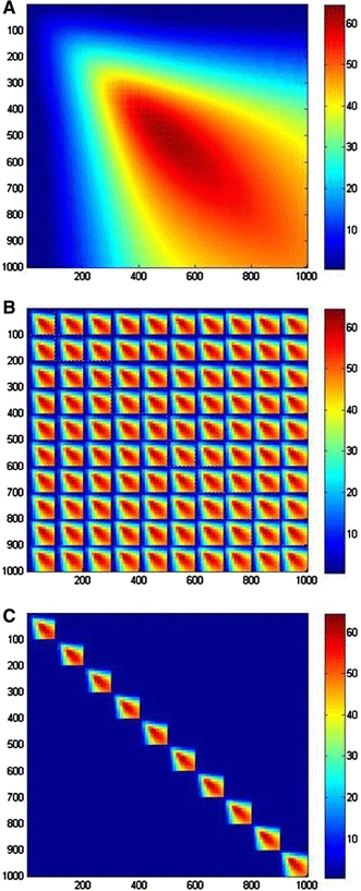
Magnitude of the elements of the normal matrix P calculated for the 10 × 100 model shown in Fig. 1. P is symmetrical and has 1,000 × 1,000 values, plotted here by row and column numbers as indicated in the abscissa and ordinate of the picture, and the values  are plotted using the color scale. In principle, the nomenclature indexing the 10 × 100 grid points for the f
r × s grid to form the vector of 1,000 parameters is arbitrary. a Here, all grid points are sorted by increasing s-value, i.e., (s
1, f
r,1), (s
1, f
r,2),…(s
1, f
r,10),(s
2, f
r,1),…(s
2, f
r,10),…(s
100, f
r,10). As can be discerned from the smooth appearance, the matrix elements are not strongly dependent on the f
r-value. b The same matrix can be reordered to reflect subdivision along ten regular subgrids γ, each of the form (s
10(γ−1)+1, f
r,1), (s
10(γ−1)+1, f
r,2),…(s
10(γ−1)+1, f
r,10), (s
10(γ−1)+2, f
r,1), (s
10(γ−1)+2, f
r,2),…(s
10(γ−1)+2, f
r,10),…(s
10(γ−1)+10, f
r,1), (s
10(γ−1)+10, f
r,2),…(s
10(γ−1)+10, f
r,10) with γ = 1…10. Each of the subgrids represents an evenly spaced 10 × 10 grid with origin shifted by Δ2
s = 0.1505 S. c The idea that one could determine a high-resolution size-and-shape distribution from merging the results obtained separately in fits with subgrids corresponds to the assumption that there be no correlation between points from the different grids, i.e., that P can be subdivided into the ten submatrices P
(γ). For the present data, this corresponds to the solution of the problem with a normal matrix as shown in c. Clearly, this is very different from the true matrix shown in b
are plotted using the color scale. In principle, the nomenclature indexing the 10 × 100 grid points for the f
r × s grid to form the vector of 1,000 parameters is arbitrary. a Here, all grid points are sorted by increasing s-value, i.e., (s
1, f
r,1), (s
1, f
r,2),…(s
1, f
r,10),(s
2, f
r,1),…(s
2, f
r,10),…(s
100, f
r,10). As can be discerned from the smooth appearance, the matrix elements are not strongly dependent on the f
r-value. b The same matrix can be reordered to reflect subdivision along ten regular subgrids γ, each of the form (s
10(γ−1)+1, f
r,1), (s
10(γ−1)+1, f
r,2),…(s
10(γ−1)+1, f
r,10), (s
10(γ−1)+2, f
r,1), (s
10(γ−1)+2, f
r,2),…(s
10(γ−1)+2, f
r,10),…(s
10(γ−1)+10, f
r,1), (s
10(γ−1)+10, f
r,2),…(s
10(γ−1)+10, f
r,10) with γ = 1…10. Each of the subgrids represents an evenly spaced 10 × 10 grid with origin shifted by Δ2
s = 0.1505 S. c The idea that one could determine a high-resolution size-and-shape distribution from merging the results obtained separately in fits with subgrids corresponds to the assumption that there be no correlation between points from the different grids, i.e., that P can be subdivided into the ten submatrices P
(γ). For the present data, this corresponds to the solution of the problem with a normal matrix as shown in c. Clearly, this is very different from the true matrix shown in b