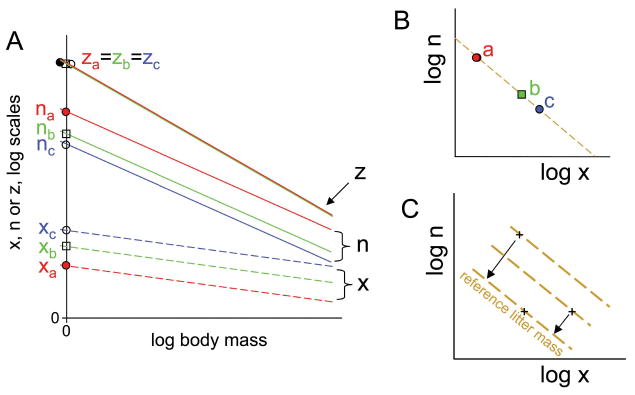
Figure 3.

Schematic illustration of our analytical methods. A, First, the allometry of each trait is analyzed in a log-log plot (as in fig. 2). Here we show three hypothetical traits, x, n, and z, in relation to body mass, indicated by dashed, solid, and dotted lines, respectively, for each of three different lifestyle groups, a, b, and c, colored red, green, and blue. The variable z represents (litter mass)/(adult mass), n represents offspring per litter, and x represents (offspring mass)/(adult mass), so for each lifestyle and for each adult mass, z = n × x and log z = log n + log x (see “Methods”). At any body mass, a, b, and c all have the same value of trait z, but a has a higher value than b or c for trait n and a lower value for trait x. The key characteristic of each lifestyle group is the relative height of its trait lines, which are indexed by their y-intercepts, here called normalization constants. B, To analyze for trade-offs between traits, the normalization constants are plotted against each other, and a trade-off between traits x and n is revealed by the negative slope. In this example, all three lifestyle groups have the same normalization constants for trait z, so their normalization constants for traits n and x lie on a straight line, shown in brown, and the labeled points satisfy the equation log z = log n + log x. In this case, the amount of resource being allocated, z, does not differ between the lifestyle groups when allometry of body mass is accounted for. C, Generally the quantity of resource being allocated differs between lifestyle groups, so the points lie on different lines. We correct for this variation by projecting trait values onto a standard reference line, as shown here.