Figure 5.

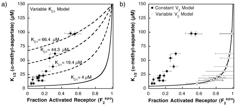
(A) Plot of the α-methyl aspartate apparent dissociation constant (K_1/2) versus the fractional activated receptor in the absence of attractant ( $F_2^{\text{apo}}$), illustrating how the K_D1 heterogeneous two-state model fits the data. Filled circles represent the experimentally determined K_1/2 and calculated $F_2^{\text{apo}}$ values for different receptor covalent adaptation states. The fractional activated receptor in the absence of attractant ( $F_2^{\text{apo}}$) was determined from equation (6) using the $V_{\text{obs}}^{\text{apo}}$ data in Table 1 and V₂ = 5.5 (see the text). The continuous curve represents the predicted behavior for a homogeneous two-state model with fixed parameters set at the most accurate current estimates (K_D1 = 4 μM and K_D2 = 150 μM). The broken lines represent a subset of the 16 curves obtained by allowing the K_D1 parameter of the heterogeneous two-state model to change with the receptor adaptation state (equation (7)) as summarized in Table 1, thereby intersecting specific data points. The broken curves shown are those that fit the QEQE modification state (K_D1 = 19.4 μM), the QQEQ modification state (K_D1 = 44.3 μM), and the QQQQ modification state (K_D1 = 66.4 μM), with fixed parameters of K_D2 = 150 μM and a relative V₂ of 5.5. (B) Plot of the α-methyl aspartate apparent dissociation constant (K_1/2) versus the fractional activated receptor in the absence of attractant ( $F_2^{\text{apo}}$), illustrating how the V₂ heterogeneous two-state model fits the data. Filled circles represent the experimentally determined K_1/2 and calculated $F_2^{\text{apo}}$ values for different receptor covalent adaptation states assuming a fixed relative V₂ of 5.5. The open circles represent a heterogeneous two-state model (equation (10)) in which the kinase activity of the activated state (V₂) is allowed to vary with the receptor adaptation state as summarized in Table 1, thereby shifting each $F_2^{\text{apo}}$ value to the right, since $F_2^{\text{apo}}=V_{\text{obs}}^{\text{apo}}/V_2$ (equation (6)). The continuous curve is the homogeneous two-state model (equation (5)) in which the microscopic parameters are fixed at the most accurate current estimates (K_D1 = 4 μM and K_D2 = 150 μM).