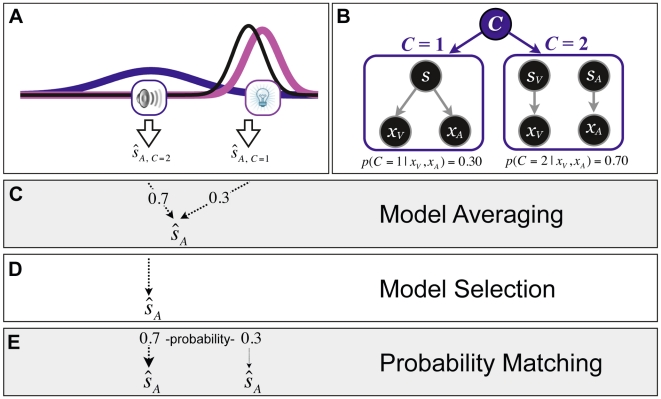
Figure 1. Illustration of the three different decision strategies for producing an auditory estimate of location.

(A) A schematic example of sensory representations on a trial with a certain discrepancy between the auditory and visual stimuli. The lightbulb and speaker symbols represent the visual and auditory stimulus locations, respectively. The visual and auditory likelihoods are shown in magenta and blue, respectively. For the sake of simplicity, here we assume that the prior distribution is non-informative (uniform). Therefore, in the case of a common cause (C = 1), i.e., when the two sensory signals are fused to obtain an estimate, a single Gaussian posterior distribution is obtained which is shown in black. The estimate of the location of sound, is the mean of the black distribution. In contrast, in the independent cause scenario (C = 2), this estimate is the mean of the blue distribution. (B) The generative model for the causal inference model. C = 1: One cause can be responsible for both visual and auditory signals, x_V and x_A. C = 2: Alternatively, two independent causes may generate the visual and auditory cues. The probability of each causal structure can be computed using Bayes' Rule (see Eq. 1). Hypothetical posterior probabilities for the stimuli in (A) are given at the bottom of each causal structure. For model averaging (C), the final auditory estimate would be a weighted average of the two estimates, with each estimate weighted by the probability of its causal structure. For model selection (D), an estimate is derived based on the most probable model, in this case the independent model (C = 2). For probability matching (E), the final auditory estimate in this example would be equal to the independent model estimate (C = 2) 70% of the time, and equal to the common cause model estimate (C = 1) 30% of the time. Visual estimates are produced likewise.