Figure 6.

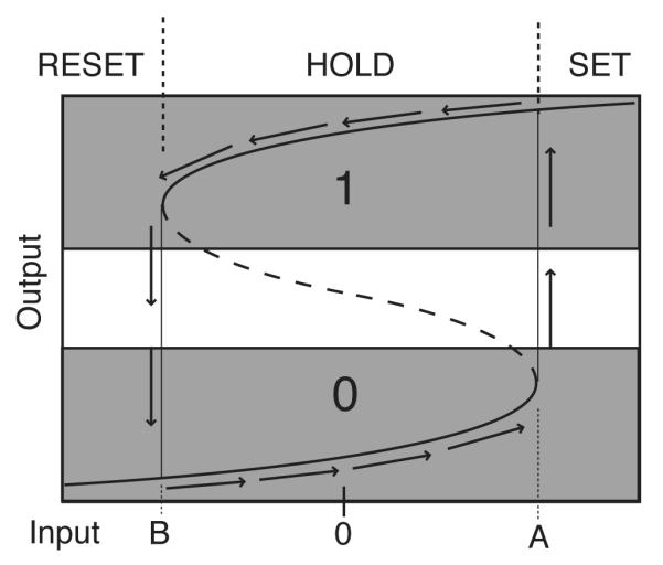
A latch based on hysteresis. The solid curves denote stable, attracting points: for any given, constant level of input, I, the system will eventually converge to a point on one of these curves centered above I on the horizontal axis. Where a dashed curve is plotted, two possible attractors exist for the same input value. Which curve the system converges to (assuming I is held fixed) is determined by the current output value of the system: if it is above the dashed curve, it will converge to the upper solid curve, otherwise to the lower curve. If the system starts out on the solid curve in the lower left corner of the diagram, and input increases, it will follow the trajectory denoted by the arrows. Input value A then defines a threshold for inputs that drive the system to a high level of output activation (corresponding to a binary 1). If inputs then drop below A, the system retains nearly maximal activation until input drops below the value B, at which point output will plunge to the lower attractor (a binary 0). It can store a 1 or a 0 as long as the input is between A and B, and will be least susceptible to noise at the midpoint between them.