Fig. 4.

Coding patterns in a network of N = 10 neurons exposed to Gaussian stimuli. (A) Uncoupled (J = 0) network. (Top) The probability distribution over response patterns {σ_i} in the absence of a stimulus. Because J = 0, this probability is uniform (for clarity, not all 1,024 values are individually shown). (Bottom) The response distributions , for two individual stimuli, red and blue; patterns on the x axis have been reordered by their to cluster around the red (blue) peak. The distributions have some spread and overlap—the response has significant variability. (B) Optimally coupled (J^∗) network that has been tuned to the input distribution. Patterns ordered as in A. (Top) Because J^∗ ≠ 0, the prior probability over the patterns is not uniform. The most probable patterns have similar likelihoods. Here, the network has “learned” the stimulus prior and has memorized it in the couplings J^∗ (see text). (Bottom) When either the blue or red stimulus is applied, the probability distribution collapses completely onto one of the two coding patterns that have a high prior likelihood. The sharp response leads to higher information transmission. (C) “Discriminability index” (DI) measures the separability of responses to pairs of inputs in an optimal vs. uncoupled network. To measure separability of responses to distinct inputs, we first compute the average Jensen–Shannon (JS) distance between response probabilities, 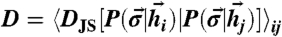, across pairs of inputs drawn independently from . Discriminability index is DI = D(J^∗)/D(J = 0), i.e., the ratio of the average response distance in optimal vs. uncoupled networks.