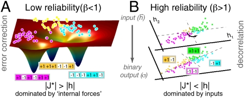
Fig. 6.

A schematic representation of the function of optimal networks. (A) At low reliability (β < 1), optimal couplings give rise to a likelihood landscape of network patterns with multiple basins of attraction. The network maps different N-dimensional inputs {h_i} (schematically shown as dots) into ML patterns —here, magenta, yellow, and cyan 6-bit words—that serve as stable representations of stimuli. The stimuli (dots) have been colored according to the that they are mapped to. (B) At high reliability (β > 1), the network decorrelates Gaussian-distributed inputs. The plotted example has two neurons receiving correlated inputs {h₁,h₂}, shown as dots. For uncoupled networks (upper plane), the dashed lines partition the input space into four quadrants that show the possible responses of the two neurons: {-1,-1} (magenta), {-1,1} (cyan), {+1,+1} (green), and {+1,-1} (yellow). The decision boundaries must be parallel to the coordinate axes, resulting in underutilization of yellow and cyan, and overutilization of magenta and green. In contrast, optimally coupled networks (lower plane) rotate the decision axes, so that similar numbers of inputs are mapped to each quadrant. This increases the output entropy in Eq. 6 and increases the total information.