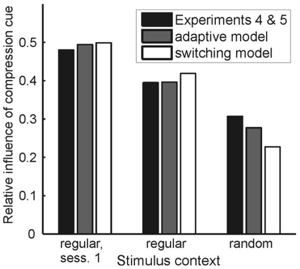
Figure 10.

Performance of Bayesian adaptive models. Shown here are the average compression cue weights derived from simulations of the two adaptive models discussed in the text for the three stimulus conditions in Experiments 4 and 5. The first is a continuous adaptive model that estimates the proportion of isotropic figures in the current stimulus set based on the assumption that it changes continuously over time as a random walk (gray bars). The second is a model that assumes that the proportion of isotropic figures changes at random, discrete moments in time, and when it does, can change to any value between 0 and 1 with equal probability. The parameters for the models simulated here were σ_jump = 0.05 for the continuous adaptive model and p_jump = 1/30 for the switching model. 100 model “subjects” were simulated, estimating slant for random sequences of stimuli generated using the same generator function used for Experiments 4 and 5. The models took as input on each trial estimates of stimulus figure aspect ratio (in the image) and slant-from-disparities corrupted by Gaussian noise with the variance parameters used for the Bayesian estimators. Results shown here are the average compression cue weights derived from the model subjects’ estimates of slant in each of the three conditions of the experiment. The black bars show average compression cue weights for the “real” subjects in Experiments 4 and 5, since subjects in the two experiments showed no significant differences in performance.